5. Noise

Grass, smoke, coastlines, and a hand-drawn line all vary smoothly, and random only knows how to jump. The function that varies smoothly is noise, and this chapter teaches it from a single drift to layered fields that change with time and loop. The meadow above is fifteen hundred blades combed by one wind, all grown from that function. Other fields follow it, built by other rules: triangles, cells, folds, and warps.

Random that remembers: noise

Here is the difference in one picture. Both strips march across the canvas asking for a height at every step. The top one asks random, and every answer stands alone. The bottom one asks noise, and something new happens: nearby questions get nearby answers.

That is the whole idea. noise takes a number in and hands back a value between 0 and 1, like random() does. But it is a lookup. At launch a smooth invisible landscape is laid out, and noise(x) reports its height at position x. Ask at 2.00 and then at 2.01 and you get almost the same answer, because you asked almost the same place. Ask far apart and the answers are unrelated. Random forgets; noise remembers where it is.

Here it is in motion. Make MySketches/Glide.swift:

import Ollin

final class Glide: Sketch {
    override func draw() {
        background(Color(hex: 0x0E1116))
        noStroke()
        fill(Color(hex: 0x64DFDF))
        let y = noise(time * 0.4) * height
        drawCircle(width / 2, y, 44)
    }
}

The dot floats up and down. There is no rhythm you can predict, but there is also never a jolt. The input is time * 0.4, so the dot is strolling along the landscape at 0.4 units a second and reporting the terrain as it goes. Now swap noise for random() (drop the argument) and run it again. The dot teleports every frame. The range and the canvas are the same, and the feel is completely different. Put noise back.

One habit carries over from Chapter 4. The landscape is laid out from the sketch's variation at launch, so every run strolls different hills. noiseSeed(6) pins the landscape, and seed(6), which you met in Chapter 4, pins noise and random together. The same seed gives the same hills.

Drift that swings: signedNoise

Chapter 4's grid nudged its corners with random(-1, 1) scaled by an amount, a swing both ways. Noise has the same convention built in. signedNoise is the same landscape spoken in -1...1, for when the natural resting point is a center rather than a floor. In Glide, replace the two lines that place the dot:

let x = width / 2 + signedNoise(time * 0.3) * 300
let y = height / 2 + signedNoise(time * 0.3 + 500) * 300
drawCircle(x, y, 44)

You get a dot wandering around the center, drifting up to 300 pixels in any direction and always coming back. There is a small trick in the second line. Both coordinates stroll the landscape at the same speed, but 500 units apart, and places that far apart are unrelated terrain. So x and y drift independently from one shared landscape. Whenever you need several unrelated glides, ask one noise in several far-apart places rather than reaching for several noises.

The zoom multiplier

The * 0.4 in Glide and the * 0.3 after it are the number that sets a noise's scale. The input to noise is a position, so the multiplier decides how far apart your questions land on the landscape:

Tiny steps stay on one hillside, so the result glides. Bigger steps cross whole hills between asks, so the result gets busy. Steps that are too big land on unrelated terrain every time, and noise stops looking smooth at all. If your noise ever looks like static, your multiplier is too big.

The panels suggest a working range. When you feed noise pixel coordinates, which you are about to, multiply them by something small, usually between 0.001 and 0.02. A 1080-pixel canvas times 0.006 spans about six of the landscape's hills: features big enough to read as shapes, small enough to be interesting. You tune this by eye, and it is easier to tune once you think of it as zoom.

Two dimensions: a field

Here is where noise does what Chapter 4's rolls could not. Give it two numbers, noise(x, y), and the landscape becomes a smooth surface: an answer at every point of a plane. Ask at every cell of a grid and you can see it:

Make MySketches/Clouds.swift:

import Ollin

final class Clouds: Sketch {
    override func setup() {
        noiseSeed(6)
        noStroke()
    }

    override func draw() {
        let cells = 45
        let cell = width / Double(cells)
        for row in 0..<cells {
            for col in 0..<cells {
                let x = Double(col) * cell
                let y = Double(row) * cell
                let n = noise(x * 0.006, y * 0.006)
                fill(Color(white: n))
                drawRect(x, y, cell, cell)
            }
        }
    }
}

That is clouds, in about twenty lines. Each cell asks the field at its own position, times the zoom multiplier, and paints the answer as a gray. Color(white:) runs from 0, black, to 1, white. Neighboring cells ask neighboring places, so the shades drift instead of flickering, and cloudy continents appear. The right panel of the figure is the same field with its answers drawn as dot sizes instead. That pointillist look is a two-line change: a fixed fill, and a drawCircle sized by n. This move, compute a value per position and let it drive any visual property you like, is most of what noise is for.

The third dimension is time

The Clouds field holds still. To move it, ask for one more dimension. noise(x, y, z) is a smooth volume of answers. Slide z gently while keeping x and y put, and every point of your 2D field changes, smoothly, each at its own pace. In Clouds, change one line:

let n = noise(x * 0.006, y * 0.006, time * 0.15)

The clouds become weather. Nothing scrolls, since sliding x instead of z is what does that. The field boils in place, the way clouds do. The 0.15 is the zoom multiplier again, pointed at time, so smaller drifts slower.

Coming home: the loop: argument

A drift that never returns cannot loop, and Chapter 3 taught you to care about that. A z that grows with time never comes back to where it started, so this weather cannot close a GIF loop on its own. You could fold time with Chapter 3's pingPong, and out-and-back does loop. But then the weather spends half of every lap running in reverse. Noise has a better answer built in. Walk a circle through the field instead of a straight line and you end where you began, facing the way you started. There is no reversal and no seam. That is the loop: argument. In Clouds, change the same line again:

let n = noise(x * 0.006, y * 0.006, loop: loopProgress(over: 4), radius: 0.6)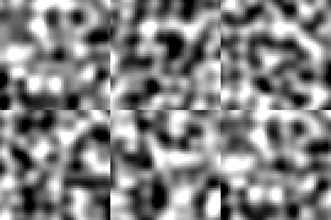

loop takes a 0...1 progress, which Chapter 3's loopProgress makes a four-second one here. One lap of it tours a closed circle through the field, and radius sets how much terrain the lap covers, so bigger is windier weather. The figure is this move, and it loops because of it. Inside, the circle runs through two extra noise dimensions, inputs beyond the ones you draw with, a trick the looping-GIF artists use. The Noise reference has the details, including using loop: to close a wave around a ring in space. A whole volume loops the same way. noise(x, y, z, loop:) reads a 3D field that comes home every lap, for a point cloud's drift or a block of turning boxes. The HiddenLines example turns ten thousand boxes by it.

The same circle is built into the sway from Chapter 3. Its .wander shape reads the noise field instead of a curve, so it never repeats inside a lap. It walks a closed circle like this one, so it still arrives home at the end of the lap:

drawCircle(width / 2, height / 2, sway(over: 4, in: 100...300, shape: .wander))

Layering shape and detail: fbm

Look at a mountain ridge and there are two ridges: the huge slow silhouette, and the small jagged texture on top of it. One noise call gives you one or the other, never both, because one zoom level only has features of one size. The fix is to ask twice and add:

let n = noise(x * 0.004) * 0.7 + noise(x * 0.03) * 0.3

The big-scale sample carries most of the weight and decides the composition. The small-scale sample gets the rest and supplies the grain. The weights should sum to about 1 so n stays in 0...1. Graphics people call these layers octaves and stack four or five of them, each layer half the size and half the weight of the last. The technique's name is fractal noise, and it is two lines of arithmetic.

Ollin also packages the stack as one call, fbm. The name is short for fractional Brownian motion, the mathematical name for this kind of layering. fbm(x * 0.004) layers four octaves, each half the size and half the weight of the one before, and still fills 0...1. Three arguments tune it. The octaves: argument is how many layers. The gain: argument is how fast the weights shrink, and lacunarity: is how fast the features shrink. fbm(x, octaves: 1) is plain noise again, so there is nothing new to unlearn. It comes in the same shapes as noise does, such as fbm(x, y) and signedFbm. There is also fbm(x, y, loop:), for layered weather that comes home each lap.

Putting it together: a meadow in the wind

The meadow at the top of this chapter puts a noise field, time, and layering to work on about 1,500 blades. Each blade grows the way Chapter 4's walker walked, one step at a time, except that its steps do not jump at random. At every step it asks a signedNoise field which way to lean. Nearby blades ask nearby places, so they lean together, and currents appear. A second, bigger-scale ask decides each blade's color and thickness, the layering idea working as composition. And the whole field uses loop:, one lap of wind every six seconds, so it sways forever without a seam. One call is new here, strokeCap(.round), which rounds the ends of every line so six short segments join into one blade. Make MySketches/Meadow.swift:

import Ollin

final class Meadow: Sketch {
    @Param("Sway", 0...1) var sway = 0.55
    @Param("Glow", 0...1) var glow = 0.4

    let ramp = Ramp([
        Color(hex: 0x11553F), Color(hex: 0x2A9D8F),
        Color(hex: 0x8AB17D), Color(hex: 0xE9C46A),
    ])

    override func setup() {
        noiseSeed(11)
        strokeCap(.round)   // segments overlap their joints into one blade
    }

    override func draw() {
        background(Color(hex: 0x0E1116))
        noFill()
        randomSeed(3)                          // the same planting every frame
        let up = -Double.tau / 4
        let breeze = loopProgress(over: 6)     // one lap of wind per six seconds

        for row in 0..<38 {
            for col in 0..<40 {
                let x = 45.0 + Double(col) * 26 + random(-1, 1) * 8
                let y = 95.0 + Double(row) * 26 + random(-1, 1) * 8
                let weather = noise(x * 0.0011, y * 0.0011, loop: breeze, radius: 0.5)
                let blade = ramp.color(at: weather)
                strokeWeight(1.5 + weather * 2.3)

                var px = x, py = y
                for segment in 0..<6 {
                    let angle = up + signedNoise(px * 0.0016, py * 0.0016, loop: breeze, radius: 0.5) * 1.15 * sway
                    let nx = px + cos(angle) * 8
                    let ny = py + sin(angle) * 8
                    stroke(Color.mix(blade, Color(hex: 0xFFF2CC), Double(segment) / 5 * glow))
                    drawLine(px, py, nx, ny)
                    px = nx
                    py = ny
                }
            }
        }
    }
}

Run it with swift run OllinLive MySketches/Meadow.swift and take it apart:

• Chapter 4 and this chapter share the work here, so it helps to see who does what. The grid plants a blade every 26 pixels. Seeded random jitter breaks the rows, so the meadow reads as sown rather than tiled. The jitter is the random(-1, 1) * 8 pair, under randomSeed(3) so the planting holds still. Random scatters; noise flows.
• Each blade is Chapter 4's walker, minus the random step. The inner loop is the same: keep a position, step, repeat. But the step direction now comes from signedNoise at the blade's current position. So the walk is steered by a smooth field instead of jumping at random. Each of the six steps is 8 pixels long and leans up to almost a fifth of a turn off vertical at full Sway. up is minus a quarter of .tau, the angle that points straight up on this canvas. Because the field is smooth, the blade curves.
• weather is the layering idea doing the composing. It asks the same field at a coarser zoom, so it changes over broader regions. The zoom is 0.0011 against the lean's 0.0016. The weather value colors those regions warm or cool through the Ramp and thickens their strokes.
• The tip-light is Chapter 2's mixing, with each segment mixing the blade color toward warm white by Glow, brightening toward the tip.
• strokeCap(.round) is what joins the six segments into one continuous blade instead of a dashed one.
• breeze is loopProgress(over: 6) feeding both asks' loop:, so the whole field tours one closed circle through the noise every six seconds. The wind never reverses and never jumps, and any six-second export loops. Both asks share the same lap but different spatial scales, which is why color-weather and lean-weather move together without being copies.

When it feels right, export it. Video keeps the most quality, while a GIF loops anywhere you paste it (trim its width and frame rate, since meadows make heavy files):

swift run OllinLive MySketches/Meadow.swift --export-video meadow.mp4 --seconds 6
swift run OllinLive MySketches/Meadow.swift --export-gif meadow.gif --seconds 6 --gif-width 420 --fps 15

Then make it yours:

• Turn Sway up to 1 and the meadow becomes kelp; near 0 it becomes fur.
• Change up to 0 and the field combs sideways into wind-swept dunes.
• Give the blades more steps, and smaller ones. Using 0..<12 with * 4 steps grows finer, longer grass.
• Swap the ramp for four colors of your own, since the weather ask does the composing either way.
• Plant sparser (* 26 up to * 40) and thicken the strokes for a reed bed.

A family of fields

The meadow asked one landscape, the classic noise, at two zoom levels. Once you think of noise as a landscape you can ask, there are other landscapes, laid out by other rules. Ollin ships a small family of them. The meadow has no need for them, but a sketch that wants stone instead of clouds, or a skyline instead of hills, does. The four below all answer in roughly 0...1 and take the same zoom multiplier. The same noiseSeed pins them, so the meadow's zoom and seeding carry over unchanged.

The same idea on triangles: simplexNoise

simplexNoise is the same idea as noise, smooth and coherent. But its landscape is laid out on triangles, where the classic one is laid out on squares. The practical difference is grain. Simplex is even in every direction. The classic field carries a faint left-right and up-down bias, which you can sometimes spot in big soft washes. So simplex is the one to try when a wash looks combed. Ken Perlin designed it in 2001 as a redesign of his own function. The two take identical inputs, so trying both is a one-word edit, and signedSimplexNoise swings -1...1:

let n = simplexNoise(x * 0.006, y * 0.006)

Noise § simplexNoise is the reference, and the Randomness/NoiseKinds example puts it beside the others on one set of coordinates.

Cells from hidden points: worley

worley remembers places. It scatters one hidden point into each cell of an invisible grid. Its answer at any position is the distance to the nearest of those points. That is near zero beside a point and peaks on the walls between two. Shade the answers and the canvas divides itself into cells, a pattern that is everywhere in nature: stone, foam, cracked earth. It is Steven Worley's, from his 1996 paper on cellular textures.

let cell = worley(x * 0.02, y * 0.02)                       // stone-wall shading
let crack = worley(x * 0.02, y * 0.02, feature: .border)    // zero on the walls
let foam = worley(x * 0.02, y * 0.02, time * 0.3)           // cells that reform

The feature: argument picks the reading. The .border reading asks how much farther the second-nearest point is. That answer is zero on the wall between two cells, so small values trace the walls. Threshold it and you have cracks and veins. A jitter: of 0 pins every point to its cell center for a regular grid, while the default of 1 scatters them fully. And the third coordinate works like it does everywhere else in this chapter. Drift it with time and the cells bubble and reform in place. Noise § worley is the reference, and the Effects/Cellular example runs the same field per pixel on the GPU.

Folding the field: ridgedFbm and turbulence

Both turbulence and ridgedFbm start from the signed field and flip every dip upward. Wherever the field crossed zero, the fold leaves a sharp crease. turbulence layers those folded octaves the way fbm does. The result is billows with creased seams, the classic basis for clouds, smoke, and marble. It is as old as noise itself, from Ken Perlin's 1985 paper. ridgedFbm pushes further. It makes the creases the bright lines and lets each octave add detail only where the one below was strong. So the fine grain gathers on the crests instead of filling the valleys. A row of ridgedFbm samples reads as a mountain skyline. The ridged fold is F. Kenton Musgrave's, from his fractal terrains. Both take fbm's arguments, and both have the loop: form:

let smoke = turbulence(x * 0.004, y * 0.004)
let skyline = ridgedFbm(x * 0.004)

Noise § ridgedFbm is the reference, and the Patterns/RidgeLines example stacks ridgedFbm skylines into a landscape.

Asking the field where to ask: warpedFbm

warpedFbm samples the field at a position the field itself chose. Instead of reading fbm at your position, it first asks the field to nudge that position, then asks again, and only then reads the answer. The layers smear into flowing marble, a look no amount of plain layering produces. Domain warping as a named, shareable recipe is Inigo Quilez's, from the article Ollin's implementation follows. warp: scales the nudging: 0 is plain fbm, 1 is the classic strength, and past 1 the field tears into churn.

let marble = warpedFbm(x * 0.004, y * 0.004)

Noise § warpedFbm is the reference, and the Shaders/DomainWarp example opens up the same recipe in shader code.

Two more live in the reference. gaborNoise lays its waves at one wavelength and, if you ask, in one direction, which gives you brushed metal, wood grain, and silk. It takes pixel coordinates and a seed: of its own rather than the zoom multiplier and noiseSeed. Noise § gaborNoise has its figure and arguments, and the Effects/GaborNoise example dots the crests of the field the GPU painted. noiseFields is the whole family as a plain value that other threads can read. It is for a sketch that asks a field a few hundred thousand times a frame. Noise § noiseFields shows the call, and the Rendering/LineSpray example bends its tens of thousands of lines a frame this way.

noise and fbm cover clouds, weather, and terrain. When a sketch wants stone instead of clouds, the field for it is one of the four above. All four share the zoom, the seeding, and the far-apart places. The folded fields and warpedFbm also take loop:, while simplexNoise and worley do not.

Where this comes from

Ken Perlin built noise in 1983, after working on the computer imagery of the film TRON. He was frustrated that everything the machine made looked too clean. He published it in his 1985 SIGGRAPH paper "An Image Synthesizer." The Academy of Motion Picture Arts and Sciences gave him a Technical Achievement Award for it in 1997. It may be the only Academy Award ever won by a math function. Ollin implements his refined 2002 "improved noise" algorithm, and its simplex noise follows Stefan Gustavson's "Simplex noise demystified." The layering-octaves idea grew alongside noise in the fractal-terrain tradition. It is Benoit Mandelbrot's fractional Brownian motion, brought to graphics by the fractal-terrain artists, Richard Voss and F. Kenton Musgrave among them. Ollin's fbm keeps that tradition's name.

Daniel Shiffman's The Nature of Code and its video incarnations made noise a first-class citizen of creative-coding pedagogy, and this chapter follows them. The loop: trick tours a circle through a higher-dimensional field so a drift comes home. It was popularized by Étienne Jacob's necessary-disorder tutorials, a long series on looping-GIF craft. The family sections name their own sources: Perlin's simplex, Worley's cells, Musgrave's ridges, and Quilez's warp. The finished sketch is a near relative of the flow field, which Chapter 14 teaches in full. That technique has a generative-art tradition of its own. Full credits are in the project's attribution notes.

Go deeper

• Noise: the full reference, including the looping loop: forms, layered fbm, and the whole field family from this chapter's tour. It also covers Gabor noise, noiseFields for work off the main thread, and curlNoise, the swirling vector cousin waiting for Chapter 14.
• Random: the uncorrelated sibling, for when you want the jump.
• The family at work: Patterns/RidgeLines stacks ridgedFbm skylines into a looping landscape, and Effects/GaborNoise reads the Gabor field the GPU painted. The same fields also run per pixel on the GPU. The Effects/Cellular example is worley as a generated layer. The Shaders/DomainWarp example opens up the warp recipe in shader code. Chapter 18 teaches both.
• Appendix B draws this chapter's math, one picture per idea: Fractions, mapping, and wrapping, Noise, Fields and following them.
• Worked examples: Randomness/NoiseField (the cloud field, scrubbed by the mouse), Randomness/NoiseWave (1D noise as a wave, beside its jagged twin RandomBand), Motion/EllipseField (signedNoise driving a whole field of shapes: ellipses in one column, chord-closed arcs in the other), and Randomness/NoiseKinds (simplex, its signed reading, worley, and turbulence on one set of coordinates).
• The Molnár homage Interruptions: a field of ticks like the meadow's ancestor, its gaps carved by noise.
• The Rojo homage MexicoBajoLaLluvia: rain as a grid of small marks, colored by noise read along one diagonal. The streaks lean the way the rain falls, and slide down it over time.

Contents · Previous: Chapter 4, Randomness · Next: Chapter 6, Grids and repetition