22. Iterated forms

Take a point, apply a rule, mark where it lands, and repeat tens of thousands of times. The marks record where the point spent its time, and that record is the picture. You learn four such rules and one plotting function that draws them all. The plate above is that function called four times, each cloud condensing as its points land. Fractal flames, order turning into chaos, and questions asked of the plane one pixel at a time follow it.

The same fern, played as a game: the chaos game

Chapter 13 grew a fern by rewriting a sentence and walking it with a turtle. There is a second way to get the same plant, and it is a game of chance played with four transformations.

Each of the four rules squashes, tilts, and shifts the whole plane. One draws the fern's main body slightly smaller and turned. One draws the left frond, one the right, and one the stem. Now put a dot anywhere at all, pick one of the four rules at random, move the dot by it, and mark where it lands. Then do that again, sixty thousand times.

let cloud = ifsPoints(.barnsleyFern, count: 60_000)
    .map { Vector2($0.x, -$0.y) }        // the fern's own y grows upward
noStroke()
fill(Color(hex: 0x2E5E3A))
drawPoints(fitted(cloud, in: canvasRectangle.inset(by: .all(80))), size: 1.5)

Here is why the game draws a fern. Every one of the four rules shrinks the plane. So wherever your dot started, a few jumps later that starting position has been squashed down to nothing and forgotten. What is left is the one set of points that the four rules, taken together, map onto itself. The dot cannot leave that set and cannot stay away from it, so given enough jumps it traces the set out. The set is called the attractor, and the collection of rules is an iterated function system.

The picture also explains what the weights are for. The four rules are not picked with equal probability. The one that draws the main body is picked 85 percent of the time, which keeps the fine tip as well drawn as the base. Ollin ships .barnsleyFern, .sierpinskiTriangle, and .sierpinskiCarpet. The Sierpinski triangle is a triangle made of three half-size copies of itself, and the carpet is its square cousin. A system of your own is six numbers per rule plus a weight. Four of the six scale, turn, and shear the point, and the other two shift it, which is what makes each rule a smaller, moved copy.

ifsPoints(_:count:) plays that game for the system you name, for that many jumps, and hands back the marks as a list of points. Three practical notes come with the call. drawPoints puts one dot at every point in the list, size pixels across. The points arrive in the system's own coordinates rather than in canvas pixels, and fitted scales and centers them into any rectangle you name. The fern also needs its y negated, because it grows upward while the canvas counts downward. The points come from the sketch's own random generator, so seed from Chapter 4 makes the same cloud every run.

A formula that folds the plane: chaotic maps

The chaos game picks its next move with a coin. The second panel of the plate needs no coin at all. A chaotic map is a formula that takes a point and returns the next point, with nothing random in it. Iterate one from any start and the visits trace a shape called a strange attractor, the formula's own signature. Where the chaos game's points fill the fern evenly, these pile up. The orbit returns to some places far more often than to others, and the picture is in that unevenness. So instead of solid dots, lay every visit down faint, and let the crowded places grow bright on their own:

let map = ChaoticMap.clifford()          // x' = sin(a·y) + c·cos(a·x), y' = sin(b·x) + d·cos(b·y)
var p = Vector2(0.1, 0.1)
var trail: [Vector2] = []
for _ in 0 ..< 200_000 {
    p = map.next(p)
    trail.append(p)
}
noStroke()
fill(Color(red: 0.55, green: 0.75, blue: 1.0, alpha: 0.12))
drawPoints(fitted(trail, in: bounds.inset(by: .all(80))), size: 1)

next applies the formula once, and the loop is the whole iteration. In the comment, x' and y' are the next point's coordinates, worked out from the current x and y. map.orbit(count:) does the same loop in one call. The points live within about plus or minus two, so fitted places them the way it placed the fern. The low alpha is what makes a density plate: one dot is nearly invisible, and where the orbit returns often the dots stack. Turn the alpha up to 1 and the same points flatten into a silhouette.

For a plate with millions of visits, let the canvas keep every frame's dots. Call noClear() in setup(), as Chapter 12 did for its trails. Then draw each frame's new points with blendMode(.add) from Chapter 19. With that mode, a faint dot adds its light to what is under it rather than painting over it. Draw tens of thousands of new points a frame at a very low alpha. After a few seconds each plate holds well over a million visits:

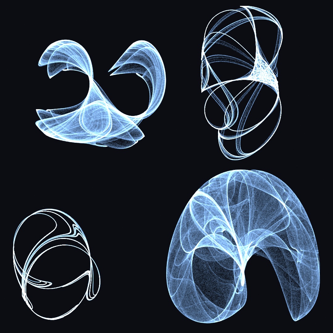
Every constant in clifford(a:b:c:d:) reshapes the form completely. Most values collapse to a dot or explode into static, and part of the craft is collecting constants that work. The four plates are four such finds, two Clifford maps above and two de Jong maps below. The same family holds .gumowskiMira(), which wanders a sea of islands into a many-petaled blossom. orbit(count:settle:) can drop the first steps of an orbit; give it none here, since the long wander is the picture. .ikeda() folds everything into one layered swirl. .hopalong() hops around nested rings that keep widening as it runs, and .henon() folds the plane into one thin bent band. The attractors reference has every form with its formula. The 3D members of this family, Lorenz and its relatives, live in StrangeAttractor and need a camera. Chapter 25 sets a million particles following one.

Circles used as mirrors: inversion limit sets

The third panel comes from a chance game again, with a different kind of move. Inverting a point in a circle turns the plane inside out around that circle. The rim stays where it is, points near the center fly far away, and points far away land near the center. The circle acts as a mirror. Take an arrangement of circles, invert the dot in one picked at random, mark where it lands, and repeat. The orbit settles onto the arrangement's limit set. The mirrors, taken together, send that set of points onto itself, the way the fern's four rules did. The one rule of the game is never to pick the same circle twice in a row. A second inversion in the same circle would undo the first.

The left panel is a fractal flame, a relative that comes after the plate. The middle panel is a ring of five circles, each touching its two neighbors, with a sixth filling the hole they leave. In canvas coordinates:

let center = Vector2(width / 2, height / 2)
let ring = 300.0, count = 5
let r = ring * sin(.pi / Double(count))
var mirrors = (0 ..< count).map { i -> Circle in
    let a = .tau * Double(i) / Double(count)
    return Circle(center: center + Vector2(cos(a), sin(a)) * ring, radius: r)
}
mirrors.append(Circle(center: center, radius: ring - r))
noFill()
stroke(Color(hex: 0x2A3242))
drawCircles(mirrors)
noStroke()
fill(Color(hex: 0xE8C97D, alpha: 0.55))
drawPoints(inversionLimitSet(of: mirrors, count: 26_000), size: 1.4)

The five centers sit on a circle of radius ring, a fifth of a turn apart. A radius of ring * sin(.pi / 5) is what makes each one touch the next. inversionLimitSet(of:count:) plays that game with the mirrors you hand it, for that many jumps, and hands back the dust as points. Since the circles are in canvas coordinates, the dust needs no fitting. It lands among the mirrors that produced it. Tangency decides the picture: circles that touch give lace, separated circles give scattered dust, and overlapping ones tear the lace apart. The points come from the sketch's random generator, like the fern's, so a seed pins them.

A group drawn as one curve: Kleinian limit sets

The last panel has no randomness in it at all. It comes from two Möbius transformations, which are the maps that send circles to circles. The group they generate is everything you can combine out of them. You apply one map, then the other, then the first one backwards, in every order and to every depth. A Kleinian limit set is the boundary all those combinations pile up against. Walking the group in order, rather than at random, traces that boundary as one line:

let curve = kleinianLimitSet(.lace)
noFill()
drawPolygon(fitted(curve.points, in: canvasRectangle.inset(by: .all(60))))

The return type is what sets this one apart from the clouds. kleinianLimitSet hands back a single Contour, the value Chapter 15 held: one ordered closed curve with roughly evenly spaced points. So it strokes, exports, and plots like any other geometry in this guide. Its points are a list of Vector2 like the other three panels' clouds, which is what lets the plate treat it the same. The right panel of the figure above is .lace, and .gasket, .cusp, and .doubleCusp are among the other presets. The Schottky entry after the plate shows the same groups as circles.

Putting it together: a plate of four orbits

Now you can build the plate at the top. It is a specimen sheet, four systems laid out under one hand, and it fills in front of you. The four steps above each made a cloud of points, and the plate composes them. The chaos game's fern and a chaotic map's orbit each get a panel. So do the dust of a ring of mirrors and a Kleinian curve's points. Each is fitted into its panel and laid down faint, a few points at a time, until the cloud is whole. One function turns a rule into a cloud of points. One other function fits that cloud into a panel and draws as much of it as has landed. Make a new file, MySketches/OrbitPlate.swift:

import Ollin

final class OrbitPlate: Sketch {
    @Param("Points per panel", 20_000...220_000) var budget = 90_000
    @Param("Dot size", 0.6...3.0) var dotSize = 1.1
    @Param("Ink", 0.05...0.6) var inkAlpha = 0.18

    let paper = Color(hex: 0x14151A)
    let ramp = Ramp([
        Color(hex: 0xE8663C), Color(hex: 0xE8B23C),
        Color(hex: 0x49B8A0), Color(hex: 0x7C6FD1),
    ])
    var clouds: [[Vector2]] = []
    var builtFor = 0

    // Six seconds of points landing, then two seconds of the finished plate.
    override var loopDuration: Double? { 8 }

    override func setup() {
        build()
    }

    override func draw() {
        if builtFor != budget { build() }
        background(paper)
        noStroke()

        // How much of each cloud has landed so far. The ease-in keeps the
        // first few hundred points on screen long enough to watch them land,
        // before the flood.
        let seconds = loopProgress(over: 8) * 8
        let grown = Easing.easeInCubic(min(seconds / 6, 1))

        let panels = grid(columns: 2, rows: 2, padding: 70, gutter: 44)
        for (index, cell) in panels.cells.enumerated() {
            let inner = cell.frame.inset(by: .all(26))
            plot(clouds[index], in: inner, ink: ramp.color(at: Double(index) / 3), grown: grown)
            label(index, in: cell.frame)
        }
    }

    // The four clouds are built once, and again only when the point budget
    // moves. The same seed makes the same clouds every time.
    func build() {
        seed(3)
        clouds = (0 ..< 4).map { orbit($0) }
        builtFor = budget
    }

    // Four rules, four clouds of points. Nothing below this line knows which
    // rule made the cloud it is drawing.
    func orbit(_ index: Int) -> [Vector2] {
        switch index {
        case 0:
            return ifsPoints(.barnsleyFern, count: budget).map { Vector2($0.x, -$0.y) }
        case 1:
            let map = ChaoticMap.clifford()
            var p = Vector2(0.1, 0.1)
            var trail: [Vector2] = []
            trail.reserveCapacity(budget)
            for _ in 0 ..< budget {
                p = map.next(p)
                trail.append(p)
            }
            return trail
        case 2:
            // A ring of mutually tangent mirrors, plus one filling their hole.
            // Tangency is the whole game: overlap them and the lace tears.
            let count = 5
            let r = sin(.pi / Double(count))
            var mirrors = (0 ..< count).map { i -> Circle in
                let a = .tau * Double(i) / Double(count)
                return Circle(center: Vector2(cos(a), sin(a)), radius: r)
            }
            mirrors.append(Circle(center: .zero, radius: 1 - r))
            return inversionLimitSet(of: mirrors, count: budget / 3)
        default:
            // A contour's points come in order along the curve. Shuffled, they
            // land all over it at once, the way the other three clouds do.
            return shuffled(kleinianLimitSet(.lace).points)
        }
    }

    // The one plotting function. Fit the whole cloud to its panel, then lay
    // down the points that have landed so far, every one at the same low
    // alpha, so that crowding is what makes a region bright. The newest few
    // go down at full ink while the cloud is still growing, so you can watch
    // the game being played.
    func plot(_ cloud: [Vector2], in frame: Rectangle, ink: Color, grown: Double) {
        let placed = fitted(cloud, in: frame)
        let landed = Int(Double(placed.count) * grown)
        let fresh = grown < 1 ? 200 : 0
        fill(ink.withAlpha(inkAlpha))
        drawPoints(Array(placed.prefix(landed)), size: dotSize)
        fill(ink)
        drawPoints(Array(placed.prefix(landed).suffix(fresh)), size: dotSize + 0.5)
    }

    func label(_ index: Int, in frame: Rectangle) {
        let names = ["a chaos game", "a chaotic map", "circles as mirrors", "a Kleinian group"]
        fill(Color(hex: 0x8A8FA0))
        textFont(OutlineFont.systemMedium)
        textSize(20)
        textAlign(.left, .top)
        drawText(names[index], frame.x + 4, frame.y + 4)
    }
}

Swift note. switch index picks one branch by a value. Each case is one value, default is every other, and a return inside a case leaves the function with that branch's answer. trail.reserveCapacity(budget) asks the list to set room aside before the loop fills it, so it never has to grow. The property clouds is a list of lists, like the trails in Chapter 10's chasers. The call (0 ..< 4).map { orbit($0) } builds it with the $0 form from Chapter 6. placed.prefix(landed) is the first landed items of a list, and .suffix(fresh) the last fresh of those. Each is a view onto the list rather than a list of its own, so Array(...) makes one again before drawPoints takes it.

Run it, then pull the ink alpha down and the point budget up. What each function does:

• build() makes the four clouds once, in setup(), and makes them again only when Points per panel moves. Building them every frame would cost the same work sixty times a second for clouds that never change. Only how much of each is shown changes. seed(3) inside it is what keeps the fern and the mirrors' dust the same from one build to the next. The mirrors get a third of the budget, since their dust crowds faster. The Kleinian curve has a point count of its own and ignores the budget.
• orbit(_:) is where the four systems live, and it is the only place they differ. Three of them return a cloud they generated. The Kleinian one returns a curve's points, which is the same list of Vector2 and so plots identically. They are shuffled first, because a contour's points come in order along the curve. In that order the panel would draw its curve from one end to the other, while the other three condense all over at once.
• loopProgress(over: 8) is the clock from Chapter 3, lapping 0...1 every eight seconds, and loopDuration declares the same eight so an export can render exactly one lap. The first six seconds grow the clouds and the last two hold the finished plate. Easing.easeInCubic shapes the growth. One second in, fewer than one point in two hundred has landed, so the first few hundred stay on screen long enough to watch, and the flood comes at the end.
• plot(_:in:ink:grown:) never asks what it is drawing. fitted measures the whole cloud and scales it into the panel, and only then does prefix keep the part that has landed. That is why the fern's own coordinates and the Clifford map's plus-or-minus-two range both land correctly, and why the picture never shifts as it fills. Fitting the landed part instead would make each cloud swell and slide as its extent grew. No numbers are set per system anywhere.
• The low alpha is the reason these read as forms rather than scribble. A single dot is nearly invisible. Where the orbit returns often the dots stack, and the density becomes the image. Turn Ink up to 0.6 and the picture flattens into a silhouette, which is the same information with the interesting part thrown away. The newest two hundred landings go down at full ink while a cloud is growing, which is what lets you see the game being played rather than a picture fading in. Once the lap holds, they go down faint like the rest.
• grid and Ramp do the layout and the color, from Chapter 6 and Chapter 2. The plate is a grid sketch that happens to be full of orbits.

Before moving on, make it yours:

• Swap ChaoticMap.clifford() for .deJong(), .gumowskiMira(), or .ikeda(). Each has its own temperament, and the panel is one word wide.
• Give the fern panel .sierpinskiTriangle or one of the other systems, and watch fitted absorb the change with no other edit.
• Feed the ring in panel three six mirrors instead of five, then let them overlap slightly. The lace tears, as the mirrors step said it would, and pulling them apart instead scatters it into dust.
• Take shuffled off the Kleinian points. That panel then draws its curve from one end to the other while the others condense, because a contour's points come in order.
• Drop to one panel at the full canvas and raise the budget to its ceiling. These are density plates, and they keep gaining from samples long past the point where a drawn shape would be finished.

The plate fills in front of you, so keep a lap of it. swift run OllinLive MySketches/OrbitPlate.swift --export-loop plate.mp4 renders exactly the eight seconds loopDuration declares, from the first landings to the held plate. For the finished plate alone, --export plate.png --frame 400 writes a frame from the hold at the canvas's full size, with the parameter values in the file.

More games with transformations: fractal flames and Schottky circles

The plate plays two chance games and walks one group. The same move, play transformations and see where the orbit lives, gives two more pictures. The fractal flame is a chaos game whose rules bend as well as squash. The Schottky circles are the paired circles behind the Kleinian curve.

The chaos game with a twist: fractal flames

A fractal flame is the chaos game with two additions. Each rule finishes with a nonlinear twist. The twist can be a swirl, a fold, or a turning inside out, so the copies are bent as well as shrunk. And instead of plotting dots, every pixel counts how many times the orbit visited it, and the picture shows the logarithm of those counts. A logarithm compresses a range. A pixel visited a million times comes out only a few steps brighter than one visited a thousand. That is what lets the blazing core and the faintest veil appear in one image. The color comes from which rules carried the orbit there, rather than from where it landed. Flames are for pictures with a range of tone no fill can give, and for watching a picture rise out of noise. The algorithm is Scott Draves's, complete by 1991, released in 1992, and written up with Erik Reckase. It ran for years as a screensaver that evolved flames by popular vote. The left panel of the figure in the mirrors step is one:

var source = SplitMix64(seed: 6)
let flame = FractalFlame.random(using: &source)
drawImage(flame.render(width: 900, height: 900, quality: 90, using: &source),
          in: canvasRectangle)

source is a random generator of your own, seeded, and handed in with & the way Chapter 4 handed randomness. quality is how many samples each output pixel gets, so a few dozen previews and a few hundred make a clean still. There is also a progressive Renderer you feed a slice of samples per frame. That is how flames are meant to be watched, rising out of the noise. Some rolls come out muddy. Reroll until one works, since that is how flames are found. Examples/Patterns/FractalFlame keeps one rising.

Circles that pair off: Schottky groups

A Schottky group starts with four circles paired two and two. A pairing is a Möbius map that turns everything outside one circle into the inside of its partner. Whatever you hand it comes back smaller, sitting in the partner. Hand a pairing the other three circles and you get three smaller circles nested inside one of them. Do it again with every pairing and its inverse, in every order, and those nest again, forever. The group is everything you can combine out of the pairings, and the lace it leaves is the group drawn at once. It is for lace you can plot, since what comes back is circles rather than dust. It is also for the family of pictures that runs from the lace to the Apollonian gasket, a disc filled with circles that all touch. Friedrich Schottky described the paired-circle groups in 1877. The way to draw them comes from Indra's Pearls, the same book the Kleinian curves come from.

let pairings = schottkyCuspedPairs(in: canvasRectangle.inset(by: .all(60)))
noFill()
drawCircles(schottkyCircles(pairing: pairings, minRadius: 0.4, maxDepth: 60))

maxDepth caps the generations, and minRadius stops a branch once its circle is too small to see, since everything below it nests inside. Whether that picture comes out full or nearly empty depends on one thing. When a pairing's two circles touch, its map holds the point where they touch perfectly still. Near that point it barely shrinks anything at all. So the orbit keeps handing back large circles generation after generation. They pile into the fan you can see at the left and right of the third panel. Separate that pair, even a little, and every application shrinks harder. The lace thins to a dust, with the same code and the same four circles.

So schottkyCuspedPairs builds its four circles as two touching pairs, and that also tells you which dial to reach for when you want motion. Its two other arguments are lean and twist. lean swings each pair around its own tangency point, so the pair goes on touching however far it swings. The picture stays full while the figure opens and closes. twist rotates a pairing off that setting, which gives spirals instead and thins the lace as it goes. SchottkyPreset names five landmark arrangements of the four circles: .kissing, .leaning, .cusped, .spiral, and .dust. schottkyCircles(.kissing, in:) takes one in place of the pairings.

What comes back is [Circle], not a cloud of points. A Möbius map sends a circle to a circle, so nothing has to be flattened on the way. The lace exports as circles, so a pen plotter draws it with the same round strokes you see on screen.

The circles and the Kleinian curves are two views of one thing, and the bridge between them is a pair of numbers. A group of this kind is picked by two numbers called its traces, and the Kleinian presets are names for pairs of them. schottkyCircles(ta:tb:in:) takes the same two traces that kleinianLimitSet takes under its preset, and builds the same group. It draws the orbit as circles, instead of tracing its boundary as a curve. At traces (2, 2) the orbit is the Apollonian gasket. Every nearby pair of traces is another member of the same family. Give a trace a second number beside its first and the packing wobbles, or loosen them and it opens.

noFill()
drawCircles(schottkyCircles(ta: Vector2(2, 0), tb: Vector2(2, 0),
                            in: canvasRectangle.inset(by: .all(60)), maxDepth: 100))

A trace is passed as a Vector2, its two numbers side by side. The complex-plane entry at the end of the chapter says what the second one means. The gasket is deep enough to want more generations than the default. The Kleinian presets name the same traces, so schottkyCircles(.gasket, in:) is this call. .gasket here and .gasket there are the same group, drawn two ways. The Patterns/Schottky example animates a small arc of this family, out from the gasket and back.

Order into chaos: the bifurcation diagram, billiards, and the double pendulum

Every system so far was plotted where its orbit went, and each settled onto one shape. The entries in this family are about when iteration stops settling. The bifurcation diagram sweeps a formula's one dial from order into chaos. A ball in a room does the same with the shape of the wall, and the double pendulum does it with nothing but gravity.

One dial away from chaos: the bifurcation diagram

A bifurcation diagram shows what a map with one dial does at every setting of the dial. Sweep the dial, let the orbit settle at each position, and plot where it landed. It is for a question the chaotic maps could not ask, since their constants were fixed: when does a formula fall apart? The one-dimensional IteratedMap family answers it. Its famous member is the logistic map, x' = r·x·(1 − x), a toy model of a population. The value x is this year's crowding, and r is how fast the population breeds. Robert May's 1976 paper in Nature made the map and its diagram famous, and the rhythm of its forks is Mitchell Feigenbaum's discovery.

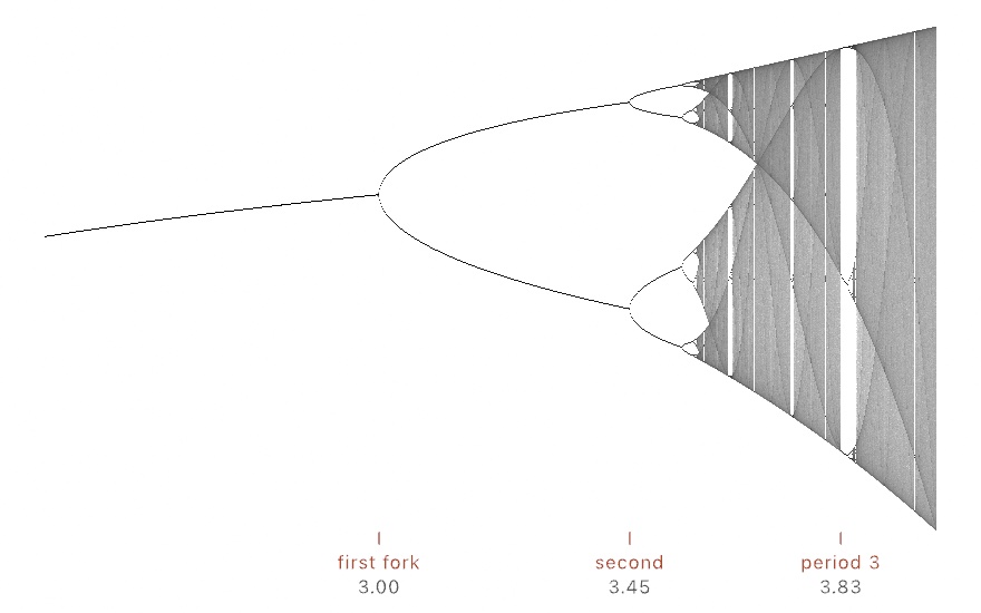
let map = IteratedMap.logistic()                            // x' = r·x·(1 − x)
let plate = map.bifurcationImage(width: 800, height: 452, samplesPerColumn: 12_000)   // sweeps r = 2.4...4

Each column of the image is one position of the dial, and samplesPerColumn is how many settled orbit points it plots. Twelve thousand, six times the default, fills the band of chaos to a smooth gray.

The diagram reads left to right like a story. At low r the population settles to one steady value, a single line. At 3 the line forks, and the orbit flips between two values forever. The forks come faster and faster until, just past 3.57, they never stop coming and the orbit never repeats again. Nothing random was added anywhere in this picture. Chaos here is a dial turned too far. The pale slots inside the gray are windows where order briefly returns. The wide one near 3.83 holds the entire diagram again in miniature. Sweep over: 3.82...3.87, the argument that sets the range of r the image covers, and see.

Two companions go with the diagram. The call cobweb(at:steps:) traces one orbit as the classic staircase between the map's curve and the diagonal. Use it to watch a single dial position. The other, lyapunovExponent(at:), scores one, where negative means settling and positive means chaos. The Examples/Patterns/Bifurcation example prints the diagram with the exponent traced beneath it, dipping below zero at every window.

A ball in a room: billiards

A billiard is the same question with no formula in it. Let a ball loose in a room. It goes straight until it meets the wall, then leaves at the angle it arrived at, forever. That is the entire rule, and it is iteration in the plainest form there is. It is for finding out how much of a picture comes from the rule and how much from the room. Billiards can answer that because here the rule never changes. The study goes back to a question of Birkhoff's. The two disorderly rooms below are Leonid Bunimovich's stadium and Yakov Sinai's square with a post in it.

let room = Billiard(.circle(Circle(center: middle, radius: 380)))
drawPolyline(room.path(from: start, heading: 0.7, bounces: 400))

middle is the canvas center and start is the point the ball is let go from, both points the sketch declares itself. Nothing changes across those four panels except the wall, and the pictures are not related.

A circle keeps a hole. Each straight run between two bounces is a chord. A bounce turns the path about the radius, which leaves untouched how far the chord passes from the middle. So every chord of the path misses the middle by the same distance. The path wraps a smaller circle it can never enter, and that circle is the hole. Every chord is the same length as every other, too, and each bounce moves the ball the same way around the rim. So a turn that is a whole fraction of a circle closes exactly into a star.

An ellipse sorts paths into two kinds. Its two foci are the two points whose distances to any point on the rim add up to the same total. The product of the distances from the two foci to a chord is the same for every chord of a path. So a path that passes between the foci keeps passing between them, and one that misses keeps missing. The two dots in the second panel are the foci, and the band is a path that never gets past them.

A stadium keeps nothing. Cut the circle through the middle and pull the halves apart, and the hole goes. The path fills the room, and two balls let go a tiny distance apart are on unrelated paths within a few dozen bounces. A post in the middle of a square does the same thing for the same reason. A round wall that curves the wrong way pulls neighboring paths apart instead of holding them together.

That last pair is the point. The rule never changed. The ball does the same thing in all four rooms. The difference between a pattern and a scribble is entirely the shape of what it bounces off. It is the same lesson as the dial above, reached from the other side.

Billiard(.stadium(center: middle, straight: 380, radius: 240))
Billiard(.polygon(walls), obstacles: [Circle(center: middle, radius: 150)])

walls is a list of a polygon's corners, the sketch's own as well. Where a ball is let go matters as much as the room. In a circle it decides how big the hole is, and a ball let go at the exact middle leaves no hole at all. room.contains(start) is the first thing to ask, since the middle of a room with a post in it is inside the post.

The classic chaos machine: DoublePendulum

A double pendulum is two weights on two rigid arms, hinged end to end, with nothing acting on them but gravity. A run of it is repeatable and impossible to predict at the same time. It is for showing that pair of facts in one picture, and for a trace that never repeats. Ollin integrates the standard equations of motion in the form Erik Neumann documents at myphysicslab, and checks itself against the energy it should be conserving. You set the arm lengths, the masses, and the starting angles. Then call advance() each frame and read bob1 and bob2, both measured from the pivot. Tracing bob2 is where the drama is.

This machine is deterministic. advance() moves one 60 fps frame on in fixed substeps, several equal small steps of the equations per frame. So a run depends only on where you started. The same start replays the same tangle every time. Start a second pendulum a ten-thousandth of a radian away, though, and within a few seconds the two are doing completely different things. That gap between perfectly repeatable and impossible to predict is what chaos means. The stadium and the gray band of the logistic map show the same gap. A fan of near-identical pendulums is the cheapest way to watch it happen. Examples/Motion/DoublePendulum draws one: twenty-four pendulums that swing as one line, then pull apart.

Iteration at every pixel: escape time, Newton's basins, and domain coloring

Every orbit so far was plotted where it went, one wandering point at a time. The other way to iterate is to give every pixel a loop of its own and ask it one question. This way of iterating is the per-pixel model of Chapter 18. Escape time asks each pixel when its orbit left. The Buddhabrot keeps the paths escape time throws away. Newton's basins ask where an orbit lands, and domain coloring asks about a single step instead of a loop. The complex-plane entry hands the arithmetic under them to a shader of your own.

Iteration without memory: escape-time fractals and orbit traps

The escape-time fractals run one small loop at every pixel: square the number you have, add a fixed one, and repeat. Some starting points stay near home forever. Others eventually run away, and the only thing the picture records is how many steps that took. That count, turned into a color, is the fractal, and the regions that never escape are the set itself, painted in one flat color, the interior: argument. They are for the boundary between the two, which holds detail at every zoom. Gaston Julia worked out the mathematics in 1918, and Benoit Mandelbrot first plotted the set that carries his name in 1980.

The loop treats a pixel's position as one number. You can add two of these by adding their coordinates, the way Chapter 10 added arrows. Squaring one is the new move. It squares the point's distance from the middle and doubles its angle around it. So a point inside the circle of radius 1 around the middle spirals inward when squared, and a point outside flies out. The fixed number added each time drags the orbit somewhere new. That is all the loop needs. The complex-plane entry, at the end of this family, draws the rule and hands it to a shader.

drawImage(generate(.mandelbrot(phase: time * 0.03)).image, 0, 0)

The first two panels are the same loop, differing only in which of its two numbers is held still. In the Mandelbrot set, the added number varies from pixel to pixel and the orbit always starts at zero. In a Julia set, that added number is fixed for the whole image, and you pass it as c. Each pixel then starts its orbit at its own position instead.

So the red mark matters. It sits at the point the code writes as Vector2(-0.79, 0.15), and the middle panel is the Julia set for that c. Move the mark and you get a different Julia set. The rule of thumb is that points near the Mandelbrot set's edge give the richest ones. Deep inside gives a plain blob, far outside gives dust. Every Julia set is a portrait of one point of the Mandelbrot set.

To mark a c on the set, hold the generator in a name and ask it for its framing. Generator is the type behind .mandelbrot() and the rest. Every generator that paints the plane hands it back as plane. Its canvasPoint(of:in:) says where a number lands in the rectangle the picture was drawn in. So a mark on a c, a root, or a zero never redoes the arithmetic:

let set = Generator.mandelbrot()
drawImage(generate(set).image, 0, 0)
if let plane = set.plane {
    drawCircle(center: plane.canvasPoint(of: Vector2(-0.79, 0.15), in: bounds), radius: 9)
}

The other way round, planePoint(at:in:) reads the number under the pointer. A sketch uses it to let you pick a c by clicking on the set.

The bands look stepless rather than like contour lines, because the coloring uses a smoothed escape count rather than a whole number. cycles sets how many times the palette repeats across the range. phase walks the colors along the bands, which is the drifting-color animation, and it costs nothing because it recolors rather than recomputes.

The third panel shows the one setting to get right:

generate(.mandelbrot(center: Vector2(-0.7463, 0.1102), zoom: 900, iterations: 400, phase: 0.4))

zoom and iterations have to climb together. The iteration cap is how long you are willing to wait before calling a point "trapped". As you magnify the boundary, more points need more steps to reveal that they do escape after all. Leave iterations at its default while zooming and the fine filigree fills in as a flat blob, because everything is being declared trapped too early. If a zoom looks like it lost its detail, raise the cap before you suspect anything else.

There is a second question you can ask the same loop. Instead of recording when the orbit escaped, record how close it ever came to a shape you hold in the plane. That is an orbit trap. Hold a cross of two lines there and every orbit that grazes it leaves a bright filament, so the picture grows stalks. Clifford Pickover introduced the trap, and the cross is his; the form used here dates to Fractint in 1989.

drawImage(generate(.orbitTrap(.cross(.zero), c: Vector2(-0.79, 0.15), zoom: 1.2)).image, 0, 0)

All three panels are the same Julia set. Only the question changes. The first asks each orbit when it escaped. The other two ask how near the cross it passed, and then turn the cross a little with angle. Feed angle your time and the stalks sweep through the filigree while the set holds still. The traps on offer are a point, a cross, a circle, and a square, and glow sets how far their light reaches. Examples/Effects/EscapeTime shows all four beside the escape-time pair, and sets a Julia's c drifting so the filigree changes shape without a break.

The escape-time picture needs no memory. Its whole loop runs inside one frame, so any frame can be computed on its own. The simulations of the next chapter iterate the other way, across frames, because their rules need neighbors and the frame before.

What the escapers leave behind: the Buddhabrot

The escape-time loop throws the escapers' paths away and keeps only a count. The Buddhabrot keeps the paths. Test random starting points, and every time one escapes, let its whole path brighten each pixel it passed through. The piled-up visits, developed like a photographic plate, form a seated figure that was hiding in the set all along. It is a density plate, like the chaotic map's, made from the orbits the Mandelbrot set rejects. It is for a picture that resolves slowly over many frames, and for false color that reads as orbit depth. Melinda Green found it in 1993, and the three-cap false-color reading is hers too.

let plate = Buddhabrot()      // three caps: long orbits red, short ones blue
let renderer = Buddhabrot.Renderer(plate, width: 560, height: 560, seed: 7)
// each frame:
renderer.accumulate(samples: 20_000)
drawImage(renderer.image(), in: canvasRectangle)

The iterations: argument of Buddhabrot, the list of caps the listing's comment names, does the coloring. Give it a single cap and the plate develops in gray. Give it three and the red, green, and blue channels expose at different orbit lengths, so color reads as orbit depth. A plate this deep resolves over many frames, the same way the flame does. Feed the Renderer a slice of samples per frame and let the figure rise. Examples/Patterns/Buddhabrot leaves one running.

Where it lands: Newton's basins

Escape time asks an orbit when it left. Newton's method asks where it ends up. The method is the step many numeric solvers take. Guess a root, which is a place where a function comes out as zero. Slide down the tangent line, the straight line that touches the curve at your guess, and guess again. Near a root it lands in a few steps. .newton runs that step from every pixel and colors the pixel by the root it reaches, so every root owns a basin. The basins are for their borders, where the method cannot make up its mind. Arthur Cayley asked what those borders look like in 1879, for a cubic, a formula built from powers of z, the pixel's number, up to the third. The color plates in Heinz-Otto Peitgen and Peter H. Richter's The Beauty of Fractals (1986) are where most people first saw the answer.

drawImage(generate(.newton()).image, 0, 0)

The left panel is the cubic with the three cube roots of one, the picture Cayley asked about. Three roots make three basins, and their borders are not straight lines. Look at the border between any two colors. The third color is there too, as a chain of beads, and each bead has the other two along its own border. Wherever two basins meet, all three do. That holds at every scale, so the boundary is dust rather than a line. It is the set of points the method never decides, folded over itself all the way down.

You place the roots yourself, up to eight. The palette spreads around them in order. shading darkens each pixel by how many steps it took, bright at the root and dark toward the edge, with a faint contour per step. phase turns the palette without recomputing anything, so it costs nothing to animate.

The middle panel changes the step. relaxation scales it. Below 1 the method creeps and the basins fatten. Above 1 it overshoots, and the basins spiral and throw off islands. Five roots at 1.3 is what the panel shows. Feed the dial a slow sine and the whole plane breathes. Examples/Effects/NewtonBasins holds the dial still and sends its roots along orbits of their own instead.

The right panel is the warning. Newton's method is not promised to land. For the cubic z³ - 2z + 2, the step sends 0 to 1 and 1 back to 0. That cycle pulls in everything near it. Those pixels are painted trapped: a large dark pool at 0 and a small one at 1. With a plain polynomial, a formula built only from powers of z, and the dial at 1, pools are rare. Move the dial and they open everywhere.

A picture of a function: domain coloring

Everything so far in this family asked a question about a loop. Domain coloring asks about a single step. A complex function takes a point of the plane and hands back another point. Graphing it the way you graph a sine wave would need four axes, two for what goes in and two for what comes out. Nobody has four axes. So domain coloring spends the two you have on the input and paints the answer as a color. The direction the answer points picks the hue, and its size waits, because direction is the part that carries the structure. It is for seeing at a glance where a function is zero and where it blows up. The method and its name come from Frank A. Farris in 1998, and the ruled forms follow Elias Wegert's phase portraits.

drawImage(generate(.domainColoring(.power(1), shading: .phase)).image, 0, 0)

The left panel is the simplest function there is, .power(1): hand back whatever you were given. Its picture is the wheel itself, and it is how you read the other two. shading: .phase asks for the direction alone. Leave shading out and rings come with it, as the paragraph on shading below explains. Red points right, and the colors run counter-clockwise from there, the way the plane is drawn on paper.

Now look at the middle panel. Two places show the entire wheel at once. The left one is a zero, where the function comes out as nothing, and the right one is a pole, where it blows up. They look alike until you follow the colors around. Then they are opposites. The wheel turns one way around a zero, and the other way around a pole. Count the wheels and you have counted the zeros and the poles. That is a theorem, drawn instead of proved, and a repeated zero draws its wheel twice.

You place them yourself, which is what lets you rearrange the field:

.domainColoring(.rational(zeros: [Vector2(-0.55, 0)], poles: [Vector2(0.55, 0)]), shading: .phase, zoom: 1.35)

Move a zero and the whole field reorganizes around it. Repeat a point for a double zero. Leave the poles out and you have a polynomial. There are named functions too: .power, .exponential, .sine, .tangent, and .logarithm. A fractional .power and the .logarithm both leave a branch cut, a line where the colors jump. The answer there had to pick one of two equally good values.

The size you set aside can come back as shading. .modulus, the default, ramps from dark to light between one doubling of the value and the next, which draws contour rings. .conformal rules the direction the same way, and the two rulings cross. That is the right panel, and close to each wheel its tiles are little squares. The squares are not a coincidence. A function like this one turns and stretches small shapes but never shears them, which would push one side past the other. The grid is that fact made visible.

phase turns the palette around the wheel without recomputing anything, so phase: time * 0.05 costs nothing and the color drifts forever. Examples/Effects/DomainColoring swims a pair of zeros around a pair of poles. The field pours from one arrangement into the next, and nothing was animated except two points.

Multiplying turns: the complex plane

The generator paints the named functions and a rational one. A function of your own is a shader, and a shader works with float2 points. Add two points and you add their coordinates. Nothing in a shader says what it means to multiply two of them, and there is no single answer. Escape time and Newton's method both lean on one particular answer, and the shader library carries it in its complex section.

The complex plane reads a point as a number, x + y·i, where i is the square root of minus one. The x part is called the real part and the y part the imaginary part, and Appendix B draws the plane. Multiplying two of these multiplies their lengths and adds their angles, and the rest of this entry follows from that one rule. It is for writing a function of the plane yourself, and for seeing why the squaring step of escape time behaves as it does. The arithmetic here follows the textbook, with one shader function per operation, after Harley Turan's walkthrough of it in GLSL.

cmul(z, z) sends every point to twice its angle, so the plane wraps around the origin twice. It also squares the length, so a point outside the circle of radius 1 moves farther out and a point inside it moves in. That is the step escape time repeats at every pixel, with a fixed number added each time. cpolar(1.0, a) builds the number of length 1 at angle a, so cmul(z, cpolar(1.0, a)) turns the whole plane by a. The other functions build on the same rule: cdiv, cexp, clog, cpow, csin, and their relatives. cdiv divides, so cdiv(z - p, z - q) in the listing below is zero at p and blows up at q. Each name matches a function on the CPU value Complex. A number you work out in draw() therefore means the same thing in a shader. The three tiles below are three such functions painted this way:

float4 shade(float2 uv, ShaderInfo info) {
    float2 z = complexPlane(uv, info.resolution, float2(0.0), 3.0);
    float2 p = cpolar(0.8, info.time), q = cpolar(0.8, info.time + 2.3);
    float2 f = cdiv(z - p, z - q);
    return float4(domainColor(f, 2, 0.7), 1.0);
}

Two helpers do the framing and the coloring. complexPlane reads the layer as a piece of the plane, with center in the middle and span units across the shorter side. The imaginary axis points up, since a uv runs down the canvas and mathematics runs up. domainColor paints the answer the way the generator did, with the direction picking the hue. The 2 asks for both rulings, the size and the direction drawn as bands, and 0.7 sets how dark they go.

The left tile is cmul(z, z), the wheel twice around, which is what adding the angles looks like. The right tile is cexp(z), the exponential function, ruled both ways. Its rulings come out straight, because the answer's size depends only on x and its angle only on y. The middle tile is the shader above, with p and q held at the angles 0.6 and 2.9 instead of turning with time. Two families of circles are drawn over it. The family nested around each point comes from draw(), worked out with Complex. Complex(magnitude:argument:) builds a number from its length and its angle, which mathematics calls its argument:

let p = Complex(magnitude: 0.8, argument: 0.6)
let q = Complex(magnitude: 0.8, argument: 2.9)
let d = (p - q).magnitude
let scale = width / 3
for n in [-2, -1, 1, 2] {
    let k = pow(2.0, Double(n))
    let center = (p - k * k * q) / (1 - k * k)     // where the ratio has size k
    let radius = k * d / abs(1 - k * k)
    drawCircle(center: Vector2(width / 2 + center.real * scale, height / 2 - center.imaginary * scale),
               radius: radius * scale)
}

Swift note. pow(2.0, Double(n)) raises 2 to the power n, so k runs through a quarter, a half, two, and four. abs is a number's size with its sign dropped. for n in [-2, -1, 1, 2] walks a list written out in place, as Chapter 16 walked its pairs.

Each of these is a circle of Apollonius, the set of points where the ratio has one size. Each is written in the same arithmetic the shader used. Drawn over the layer, each one lands on a ruling. The two halves agree, so you can reason on whichever side is easier and paint on the other. Examples/Shaders/ComplexPlane moves the two points and draws both families of circles. Two more take the same ratio somewhere else. ImaginaryLog feeds the imaginary part of its clog to a cosine palette that never completes a cycle. The branch cut between the points then shows as a soft seam. Meromorphic builds a ratio of two cubics from six moving roots and turns the palette's frequency up until the bands pile up around the poles.

Where this comes from

The plate's four systems come first. Iterated function systems and the chaos game are Michael Barnsley's, from Fractals Everywhere (1988), and the fern uses his published four-map table. The Clifford attractor is attributed to Clifford Pickover, and the de Jong attractor is named for Peter de Jong. Paul Bourke's long-running fractal pages popularized both. The Gumowski-Mira map came out of particle-beam physics at CERN, and the Ikeda map out of laser optics. Barry Martin's hopalong reached everyone through A. K. Dewdney's Scientific American column. Circle-inversion limit sets follow Michael Frame and Tatiana Cogevina's 2000 rendering method, and Frame's Yale course pages explain them clearly. The Kleinian curves come from David Mumford, Caroline Series, and David Wright's Indra's Pearls, which made Felix Klein's groups visible. The entries after the plate name their own sources. The flames and the Schottky circles name Draves and Reckase, and Schottky and Indra's Pearls again. The chaos entries name May and Feigenbaum for the diagram, Birkhoff, Bunimovich, and Sinai for the billiards, and Neumann for the pendulum. The per-pixel entries name Julia and Mandelbrot, Green, Cayley and Peitgen and Richter, Farris and Wegert, and Turan. Full credits are in the project's attribution notes.

Go deeper

• Fractals: the IFS type and its presets, the FractalFlame surface including the progressive renderer, inversion limit sets, the Kleinian trace presets, the Schottky circle orbit with both family builders and why a tangent pair keeps the picture full, and the escape-time family with its orbit traps.
• Billiards: the four rooms, letting a ball go, what each room draws and why, posts standing in a room, and drawing the room itself. The Examples/Patterns/Billiards example puts all four side by side with a fan of balls.
• Attractors: every ChaoticMap, the IteratedMap family, bifurcationImage, and the GPU tier that runs a million orbits at once. Chapter 25 puts that tier to work as a field of drifting points.
• Chaotic maps and bifurcation: the one-dimensional families, the diagram's dot and density forms, cobwebs, and Lyapunov exponents.
• The double pendulum: its settings, the energy check, and why a live deltaTime gives up the exact replay.
• Escape time, Newton's basins, and domain coloring as generators: .mandelbrot, .julia, and .orbitTrap as layers a chain can filter, with the center, zoom, iteration, and banding arguments; .newton with its placeable roots, the palette spread around them, the shading by step count, the relaxation dial, and the trapped color; .domainColoring with its placeable zeros and poles, the named functions, and the modulus and conformal rulings.
• Complex numbers: the CPU value behind the complex section, with literals, the polar form, Complex.exp and its relatives, and the Vector2 bridge. The section's own functions are on the shader library page.
• Appendix B draws the ideas under this chapter, one picture per entry: Iterated maps: orbits that pile up, Escape time, and Density as tone.
• Worked examples: Patterns/IteratedFunctions, Patterns/FractalFlame, Patterns/Buddhabrot, Patterns/InversionFractal, Patterns/Kleinian, Patterns/Schottky (the traces swung out from the gasket and back), Patterns/ChaoticMaps (the density bloom, all six presets on a parameter), Bifurcation, and Effects/EscapeTime (the pair and the four traps as generator tiles).

Contents · Previous: Chapter 21, Pictures you solve · Next: Chapter 23, Simulations on a grid