Layered effects

Draw into off-screen layers, run GPU filters over them (blur, bloom), and composite the results back onto the canvas with blend modes. That is how you build glow, soft backdrops, depth-of-field haze, and post-processing looks. The design follows the OPENRNDR compose/Filter model on Ollin's Metal core.

Everything stays on the GPU. A layer is a Metal texture you draw into and then sample. A filter reads one texture and writes another. Compositing is an ordinary drawImage with a blendMode. Nothing is ever read back to the CPU between steps. Copying a layer back to combine it is the slow path other tools fall into, and it never happens here.

override func draw() {
    background(.black)

    let layer = makeRenderTarget()                 // a full-canvas off-screen layer
    withTarget(layer) {                         // …draw into it, scoped like withState
        background(.clear)
        fill(.orange); noStroke()
        drawCircle(width / 2, height / 2, 200)
    }

    blendMode(.add)                             // add the glow as light
    drawImage(layer.filtered(.bloom(amount: 1.6)).image, 0, 0)
}

Contents

• renderTarget - make an off-screen layer
• withTarget - draw into a layer
• RenderTarget.image - composite a layer back
• filtered - run a filter over a layer
• Filter - the filter catalog (blur, bloom, color, stylize)
• combined / Combine - combine two layers (mask, displace, disperse, mix, seamless clone, defocus, ambient occlusion, screen-space reflections)
• depth - a 3D scene's depth buffer as a layer (feed .defocus / .ambientOcclusion / .screenSpaceReflections)
• generate / Generator - procedural pattern sources
• postProcess - filter the whole frame
• withOverlay - draw over the finished frame, after every pass
• feedback / withFeedback - a layer that remembers itself (trails, tunnels)
• simField / Sim - a layer that runs a simulation (reaction-diffusion, Game of Life, fluid, the self-warp motion feedback)
• Sim.shader - a simulation of your own: a kernel you write, the inject, the field's edge and precision, arrows, readback
• compose / layer - declare a stack of layers as one block
• aside - a helper layer that feeds another layer's effect
• Notes

makeRenderTarget(scale:)

Make an off-screen layer to draw into. The no-argument form is full-canvas size, and scale renders the layer at a fraction of that resolution.

let layer = makeRenderTarget()              // full canvas
let haze  = makeRenderTarget(scale: 0.5)    // half-resolution, for a layer you'll blur

Effects are fill-rate bound, because the cost tracks pixels × passes. So a layer you are going to blur or glow rarely needs full detail. Lower scale and the layer upsamples when you draw it back. There is also an explicit-size form for a layer that is not full-canvas:

let badge = makeRenderTarget(width: 256, height: 256)

Make a target inside draw(). It is a per-frame handle. Ollin pools the GPU texture behind it and reuses it across frames, so making one each frame does not allocate.

makeRenderTarget(scale:precision:) also takes a precision. The default is .float16, which is rgba16Float. Use .float32 (rgba32Float) for a layer whose values are sums or measurements rather than a picture. Half float stops moving once a step falls under about one part in a thousand of the value. Single precision costs twice the memory.

Precision follows the layer through a chain. A filter or a combine over a .float32 layer writes a .float32 layer. Every pass inside it works in single precision, and so does the next filter after it. Half float holds a distance past 1,024 pixels only to the nearest whole pixel, so a measured distance field wants this: in single precision the distance keeps its fraction to the end of the chain. A half-float layer's chain stays half float. The base of a combine sets the precision, whatever the aux holds.

withTarget(_:_:)

Redirect everything drawn in the closure into target instead of the canvas. The block is scoped exactly like withState { }. The current drawing state and transform carry in, and drawing returns to the canvas when the block ends.

let layer = makeRenderTarget()
withTarget(layer) {
    background(.clear)                  // clear THIS layer (transparent here)
    fill(.white); noStroke()
    drawCircle(width / 2, height / 2, 120)
}
// back to drawing on the canvas

Call background(_:) inside the block to clear the layer. Inside a withTarget it clears that layer, meaning its fill color and its geometry so far, and it leaves the canvas untouched. A layer starts transparent, so a layer you never wrote, or wrote only in part, composites as nothing where you did not draw.

The canvas's own background() clears the canvas and nothing else. It drops what the canvas has recorded so far this frame, and every layer drawn before it keeps its marks. So a layer, a field's seed, or a feedback loop can come before the canvas background or after it (see the frame).

RenderTarget.image

A layer as a drawable Image. You composite it with the ordinary drawImage, and it follows the transform stack, tint, and blendMode like any image:

drawImage(layer.image, 0, 0)                       // at the top-left, native size
drawImage(layer.image, 0, 0, width, height)        // scaled to fill
blendMode(.add); drawImage(layer.image, 0, 0)      // added as light

The image always shows what was drawn into the layer this frame.

filtered(_:)

Run a Filter over a layer and get back a new layer. The new layer is drawable and filterable in turn, so effects chain:

let blurred = layer.filtered(.gaussianBlur(radius: 20))
let glowed  = layer.filtered(.bloom()).filtered(.gaussianBlur(radius: 4))
drawImage(blurred.image, 0, 0)

The work runs on the GPU during the frame's render, and filtered only records it.

Filter

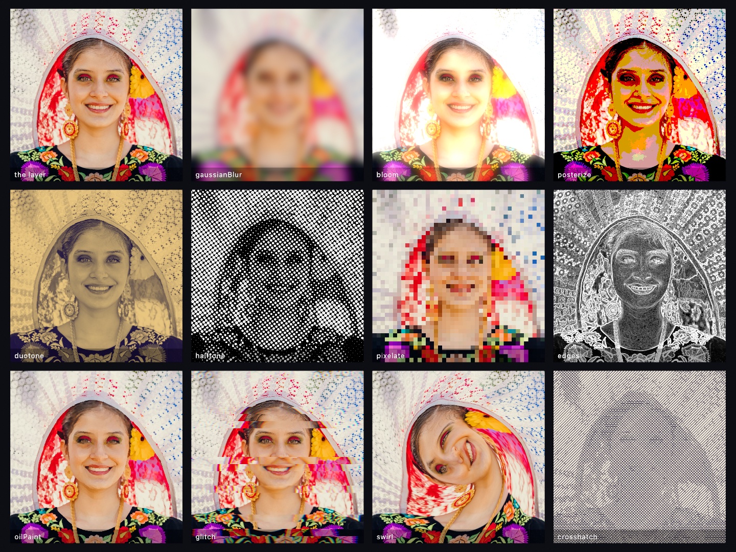
Filters are value descriptors built with static factories. They composite in linear light, so grades and blends are physically correct. Every family below is a segment of the Effects/FilterCatalog contact sheet, and Effects/Glitter shows the iridescence and glitter pair on shapes. The catalog:

Blur & glow

• .gaussianBlur(radius:) a Gaussian blur, where radius is the extent in pixels, so larger is softer. It runs on a hardware Gaussian kernel.
• .bloom(threshold:amount:radius:) glow, where pixels brighter than threshold bleed light into their surroundings. Ollin extracts the bright parts, blurs them by radius pixels, and adds them back at amount. The radius is a pixel count, not a share of the canvas: radius: 0.02 spreads nothing, and Ollin says so once when a sketch writes one. For a glow that keeps its size on any canvas, write radius: width * 0.02. The result is the original plus its glow, ready to composite, often additively. Brightness here is the max color channel (HSV "value"), not luminance, so a vivid full-brightness mark blooms the same whatever its hue. threshold runs 0…1 over the linear-light frame, so HDR highlights (values above 1, from additive light) bloom hardest.
• .halation(threshold:radius:tint:amount:) the fringe film shows around its brightest highlights. Light that gets through the emulsion reflects off the base and exposes the layers again around the point it entered, and it exposes the red-sensitive layer most, since that one sits deepest. The pixels above threshold (the max channel over the linear-light frame, as .bloom reads it) are blurred by radius pixels, colored by tint (a warm orange by default), and added back at amount. What sets it apart from a glow is where the halo lands. Scattered light changes nothing in a layer that is already fully exposed, so each channel takes the halo in proportion to how far it sits below white. A white core stays white and gets a warm ring. A mid-tone beside a highlight takes the whole tint, and a frame with nothing above the threshold comes back byte for byte. The halo is the blurred highlight times the tint. So tint: .white keeps each highlight's own color in its fringe, which is the look a saturated scene wants, where the default dyes every fringe the same orange-red. See the Effects/FilmLook example.
• .bilateral(radius:sigma:) edge-preserving smoothing that blurs flat areas while keeping edges sharp, the base for a cartoon or a denoise look. sigma is how different a neighbor's color may be before it stops blending, so a smaller value keeps more edges.
• .motionBlur(angle:distance:) a directional smear along angle, where distance is a fraction of the layer. It gives you the streak of a moving subject.
• .radialBlur(amount:) a zoom blur smearing outward from the center, where amount is a fraction of the layer.

layer.filtered(.gaussianBlur(radius: 24))
layer.filtered(.bloom(threshold: 0.6, amount: 1.4, radius: 24))
layer.filtered(.halation(threshold: 0.8, radius: 24))
layer.filtered(.bilateral(radius: 6, sigma: 0.18))

Layer styles

• .outline(width:color:align:), .dropShadow(offset:radius:color:), .innerShadow(offset:radius:color:), .outerGlow(radius:color:), .innerGlow(radius:color:), and .bevel(width:depth:profile:angle:elevation:highlight:shadow:) give a layer an edge of its own, read from its alpha. Each is one filter, and chained styles stack in the order they run. Layer styles covers each one, how they stack, and how exact they are.

layer.filtered(.bevel(width: 14)).filtered(.outline(width: 6, color: .black)).filtered(.dropShadow())

Color & tone

• .colorGrade(brightness:contrast:saturation:hue:) the everyday grade. It takes an additive brightness and a contrast that pivots on mid-gray. It also takes a saturation (0 = gray, >1 = punchier) and a hue rotation in turns (0…1 wraps the wheel). All four default to no change, so pass only the ones you want.
• .invert(amount:) move the colors toward the photographic negative, where amount 1 is the full negative.
• .posterize(levels:) quantize each channel to flat steps, for the banding of a screen print.
• .threshold(_:softness:) cut the layer to two tones at a brightness, where softness widens the edge.
• .sepia(amount:) a warm monochrome tone, blended by amount.
• .channelMixer(_:) every channel of the result is a weighted sum of the input's red, green, blue, and alpha plus an offset, read off a ColorMatrix: the channel mixer of a photo tool, with the alpha row in play too. ColorMatrix.gray mixes the display's own gray (the BT.709 weights, in linear light), ColorMatrix.gray(red:green:blue:) a gray to a recipe (a black-and-white photographer's red filter is gray(red: 0.6, green: 0.3, blue: 0.1)), ColorMatrix.swapping(_:_:) trades two channels named by ColorMatrix.Channel (.red, .green, .blue, .alpha), and ColorMatrix.identity changes nothing. A matrix built by hand is ColorMatrix(red:green:blue:alpha:), one row per output channel, each [r, g, b, a, offset]; a row left out keeps its channel, a short row reads its missing entries as zero, and values holds the twenty numbers row by row. The multiply runs in linear light on the straight color, so a half-transparent layer keeps its edges, and the identity matrix changes no byte. It crosses to the web page.
• .duotone(dark:light:amount:) map luminance between two colors (shadows → dark, highlights → light).
• .gradientMap(_:amount:) read luminance and look its color up along a Ramp or Colormap (viridis, magma, turbo, …). It is a fast way to recolor a grayscale field or a whole scene.
• .lut(_:amount:) move every color through a ColorLUT, the table a grading tool exports as a .cube file (a film look, a grade, a print emulation) or one built in code. The table is read on the encoded picture, a cube by tetrahedral interpolation, and amount fades it in. A curves table crosses to the web page; a cube stays with video. See Looks.
• .softProof(_:warning:amount:) show the layer as a press will print it, through an ICC profile. The colors ink cannot reach are pulled in, and the blacks are lifted to what ink can do. warning paints what will not survive in that color instead, and amount: 0 leaves the colors alone so only the flag shows. See Print color.
• .exposure(stops:) scale the light in linear-light stops (+1 doubles, −1 halves).
• .develop(exposure:ground:) print a layer of accumulated light. The layer is scaled by exposure, rolled off through the Reinhard curve, and laid on ground. The ground is added after the curve as a display color, and written as the display value itself. This is what an Accumulator's developed runs. See Depth of field from light.
• .levels(blackPoint:whitePoint:gamma:) the levels control of a photo tool. It pulls blackPoint to black and whitePoint to white, then bends the midtones by gamma (>1 darkens).
• .solarize(_:softness:) invert the tones above a brightness with a soft fold, for the part-positive, part-negative darkroom look (the Sabattier effect).
• .temperature(amount:tint:) white balance: amount warms (>0) or cools (<0), tint pushes toward magenta (>0) or green (<0).
• .vibrance(amount:) saturation that lifts the muted colors most and the vivid ones least. It strengthens a flat image without blowing out tones that are already saturated.
• .colorama(cycles:shift:) cycle the hue wheel cycles times across luminance, turning a gradient into rainbow bands, and shift spins the wheel.
• .lumaKey(low:high:inverted:) a luminance key. It makes the image transparent outside a brightness band, so a dark or light backdrop drops out.

layer.filtered(.colorGrade(contrast: 1.3, saturation: 1.6, hue: 0.05))
layer.filtered(.channelMixer(.swapping(.red, .blue)))
layer.filtered(.channelMixer(ColorMatrix(red: [1, 0, 0, 0, 0.1], blue: [0, 0, 0.8])))
layer.filtered(.gradientMap(.turbo))
layer.filtered(.lut(.warmPrint, amount: 0.8))
layer.filtered(.levels(blackPoint: 0.08, whitePoint: 0.92, gamma: 1.4))
layer.filtered(.vibrance(amount: 0.6))

Stylize & optical

• .arrows(spacing:scale:color:width:) a two-channel layer drawn as arrows: the picture of a wind, a gradient, or any field whose red is an x and green a y. One arrow per cell of spacing pixels reads the vector at the cell's center in the layer's own units, times scale into pixels, and draws it from that center as a shaft with two barbs, width pixels wide, in color. A vector longer than the spacing is cut to it, so the arrows say direction and scale says how much of the size is shown, and one shorter than half a pixel draws nothing. The result is ink over transparency, so it composites over the field it reads or over anything else. Its usual partner is a Sim.shader field holding a velocity, and the Simulation/Wind example draws one that way.
• .antialias(amount:threshold:quality:) smooth the stair-stepped edges of a layer that a fragment shader wrote pixel by pixel. Ollin anti-aliases the shapes you draw. A generate(_:) pattern, a raymarched field, an imported shader, or a finished chain is different. Each writes a final color per pixel and carries no coverage, so a hard edge inside one comes out as a staircase. This pass works from the image alone. It finds each edge by brightness, follows it to both ends, and reads the layer back a fraction of a pixel across it. That turns the steps into a ramp.

threshold is the contrast an edge needs before the pass touches it at all. A lower value reaches fainter edges and costs more, and a layer with nothing over that contrast comes back byte for byte. quality is how far the pass may follow one edge. amount is how much of the result to keep, so amount: 0 hands the layer back unchanged.

It reads pixels rather than shapes, and that sets what it can do. It cannot tell a stair-step from detail that is genuinely one pixel wide, so it softens both. That is why you place this filter yourself instead of every layer getting it. Place it right after whatever wrote the layer, and before a warp that would smear the ramp it just made. On a measured shallow edge it halves how far the edge strays from the straight line it should lie on. Half rather than none is what a pass reading the finished image can do. See Examples/Effects/Antialias.

• .edges(amount:) Sobel edge magnitude, drawn as bright edges on black. It is a quick ink or outline pass.
• .sharpen(amount:) an unsharp mask, which emphasizes local detail.
• .vignette(amount:radius:softness:) darken toward the corners. It is aspect-correct, so the darkening stays circular.
• .chromaticAberration(amount:mode:spectral:quality:) pull the color channels apart, the way cheap glass, a misprinted plate, or a lens wide open does. amount is the split in fractions of the canvas. mode picks which picture you get, because the members of this family look unlike each other rather than like one look at different strengths:

• .magnify (the default) scales each channel about the center. Nothing splits in the middle, the split grows in step with the distance out, and straight lines stay straight. This is the physically honest form of lateral color.
• .lens(radius:falloff:) shapes that growth. radius (0…1 of the half-diagonal) is where the fringe starts to show at all. falloff is the exponent it grows by past there, and about 2 reads like glass. .lens(radius: 0, falloff: 1) is .magnify again.
• .offset(angle:) moves every pixel by the same vector, so the middle splits as much as the corner. This is misregistration rather than optics: a plate printed a hair off, an anaglyph, or a scan that slipped.
• .edges fringes only where there is an edge. It slides along the local brightness gradient and scales by how strong that gradient is, so flat regions keep their exact color. A positive amount leaves a warm halo on the bright side of every edge, and a negative one leaves the cool, purple-fringing kind.
• .axial is longitudinal color. The channels differ in focus rather than in position, so one end of the spectrum is sharp while the other softens. A positive amount keeps red sharp and a negative one keeps blue sharp. That is what turns an out-of-focus highlight green on one side of focus and magenta on the other. It carries most of the look of a fast lens wide open, and it pairs with .defocus rather than replacing it.

spectral: true takes the split over a whole set of wavelength taps rather than three, which turns three hard ghosts into a continuous rainbow smear. quality sets how many taps (7 / 15 / 31). This is the largest single jump in quality here. It is off by default, because three taps give the cheap glitch look people often want. Every mode hands the layer back untouched at amount: 0, so an A/B costs nothing. Each tap is unpremultiplied before its channel is read. A layer with soft edges of its own then keeps them instead of growing a dark rim. Past the frame edge the sampler clamps. See Examples/Effects/Dispersion, and use .disperse to drive the amount from a second layer.

• .halftone(scale:angle:) a rotated dot screen, dot size tracking brightness.
• .dither(levels:) ordered dithering (Bayer 4×4), the retro look that fakes more shades than it has.
• .dither(dark:light:bias:pixelSize:) the two-tone variant. The same ordered pattern is mapped onto exactly two chosen colors and cut by tone, which gives the 1-bit or newsprint look in any palette. bias shifts the cut (positive lightens), and either color may be transparent so the shadows drop out.
• .grain(amount:seed:) per-pixel noise, the same at every tone, so feed seed your time or frameCount for noise that moves. It clamps at black, so a black field comes up as a scatter of specks; for a grain that leaves black black, use .filmGrain.
• .filmGrain(amount:size:seed:) the grain of a film stock. A developed frame is a scatter of grains, so its noise follows the tone: none where nothing developed, none where every grain did, most in the middle. Each channel is perturbed by amount times the square root of its tone times what is left to white, on the displayed picture rather than in linear light, so amount is the grain's spread at mid-gray as a fraction of the way to white (0.05 is about twelve levels of a display byte). size is how many pixels across a grain clump is, and the spread is the same at any size, so a coarser grain is not a fainter one. The mean of a flat region is kept, so grain never lifts or darkens a picture, and a value above white keeps its excess. seed picks the pattern; feed it frameCount for the fresh grain every frame of a film has. Black and white take no grain at all, byte for byte. The spread grows as the square root of the tone, so relative to the tone it is largest in the darkest shades. A near-black area shows the speckle first, while a true black stays clean and the frame's mean holds. To quiet the shadows, lower amount. See the Effects/FilmLook example.
• .pixelate(size:channel:tint:) mosaic into blocks size canvas-pixels across, where channel can read one channel out as gray and tint can recolor it.
• .lineScreen(scale:softness:angle:foreground:background:) a brightness-driven line screen. Each cell paints a centered bar whose width tracks that cell's brightness, in foreground over background.
• .emboss(amount:angle:) light the luminance slope along angle as a gray relief, like stamped metal.
• .oilPaint(radius:) the Kuwahara region filter. It flattens detail into oil-paint patches while keeping edges crisp. radius is the brush size in pixels, so bigger is broader and costs more.
• .brushwork(radius:stretch:sharpness:) the picture as paint laid on in patches that follow its own flow, the anisotropic Kuwahara filter. Each pixel becomes the average of the flattest of eight overlapping sectors of a brush around it, so detail flattens into patches while edges stay crisp. The brush is an ellipse drawn out along whatever edge runs through the pixel. So the patches read as strokes along the picture's contours rather than the square dabs of .oilPaint. radius is the brush size in pixels, and the cost grows with its square. stretch is the most the brush is elongated along an edge, as an aspect ratio. 1 keeps it round, and the default of 4 is the technique's own tuning. sharpness is how decisively the flattest sector wins. Higher is flatter and more poster-like, and 0 blends every sector alike, which is only a soft blur. The picture is read as the colors a display shows over white paper, so empty space on a transparent layer counts as paper, and the result keeps the layer's alpha. It runs as three passes, which the web page export does not carry. See Examples/Effects/Brushwork.
• .crosshatch(scale:foreground:background:) pencil shading, drawn as layered diagonal strokes that thicken as the image darkens.
• .hatching(spacing:length:directions:foreground:background:) the picture as pen work whose strokes follow it. The direction at every pixel is read from the structure tensor, the same flow .brushwork and .shock follow, so the marks bend around a form instead of running across it the way the fixed screen of .crosshatch does. How many go down is the picture's own tone: the ink covers about as much of the paper as the picture is dark, so the drawing holds its light and shade with nothing but line.

spacing is the distance between strokes in pixels, and so how fine the pen is. length is how far one runs before it ends, with a short length making a stipple of dashes and a long one a comb. directions is how many layers stack as the tone darkens: 1 hatches one way only, which turns the deepest tones into fat merged marks, 2 crosses the first layer at right angles once it has laid all it may, and 3 lays a third between them. The picture is read as the colors a display shows over white paper, so empty space on a transparent layer counts as paper and is left bare, and a transparent background keeps it that way in the result. The cost grows with directions times length. It runs as three passes, which the web page export does not carry. See Examples/Effects/Hatching.

• .toon(levels:edges:) cel shading. It flattens the layer into levels brightness bands and inks the Sobel edges over them.
• .xdog(radius:sharpening:threshold:softness:flow:foreground:background:) the picture as pen and ink. A line goes where the picture has an edge, solid ink where it is dark, and the rest is left as paper, in foreground over background. Two blurs of the brightness are subtracted, the smaller one radius pixels wide and the other 1.6 times that. The difference is pushed over the tone by sharpening, and the result is cut at threshold: paper above it, ink below, through a ramp softness wide. A softness of 0 is a hard two-tone print, and the default of 0.2 keeps a gray wash under the cut, which is the look the technique is known for.

The blur is taken across each edge, and its response is gathered flow pixels along it, following the edge's own direction. That is what makes the lines run continuous rather than breaking into speckle. flow: 0 leaves that out, which is worth an A/B on a noisy picture. The picture is read as its perceptual brightness over the paper. So threshold is on the 0…1 scale a display shows, and an edge in a shadow counts as much as one in the light. Empty space on a transparent layer reads as paper rather than ink. A transparent background counts as white for that reading and stays transparent in the result. It runs as four passes, which the web page export does not carry. See Examples/Effects/InkDrawing.

• .shock(iterations:flow:radius:smoothing:threshold:) the picture flattened into regions with crisp edges that follow its own flow, the coherence-enhancing filter. Each round smooths the layer along the direction of least change at every pixel and sharpens it across that direction with a shock filter. Where the brightness across an edge bends toward bright, a pixel takes the brightest pixel within reach; where it bends toward dark, the darkest. So a soft transition snaps to a step, and everything along an edge is drawn out into one coherent stroke. No color is invented: every pixel is a blend, along its own contour, of colors the layer holds.

iterations is how many rounds, and so the level of abstraction: 2 is a light clean-up, 10 a poster. flow is how far along the flow each round smooths, in pixels, adapted to how clear the direction is (a clear straight edge gets the whole reach, a flat or curved neighborhood a quarter of it). radius is how far across an edge the shock reaches, which sets the edge scale, and anything thinner than it is fattened to it. smoothing blurs the brightness the shock reads its sign from, so texture finer than it stops making edges and flattens into regions; raise it on a noisy or grainy picture, where the flow would otherwise follow the noise into a maze. threshold is the bend under which nothing is sharpened, which keeps nearly flat regions quiet. The picture is read as the colors a display shows over white paper, so empty space on a transparent layer counts as paper, and the result keeps the layer's alpha. The cost grows with iterations times flow.

• .median() a 3×3 median, knocking out speckle and stray pixels while keeping edges sharp.
• .contour(levels:amount:) dark iso-brightness lines (one every 1/levels of the range), turning tone into a topographic map.
• .cmykHalftone(scale:) separate into cyan/magenta/yellow/black and screen each as rotated dots at the classic print angles, for the color-process look.
• .normalMap(amount:) read the image as a height field and output its surface normal as an RGB vector, which gives the bluish bump-map look. The result is ready to feed .displace (see combine) or a lighting pass.
• .relight(_:angle:elevation:height:intensity:color:) read the layer as a height map (bright = raised) and light it as embossed matter with a chosen finish. The finishes are .matte clay, .metal, wet .glass, grainy .sand, and .liquid, and the last two refract the image beneath. angle sets where the light comes from, and elevation how low it rakes, so grazing light deepens the relief. height exaggerates the slopes, and color overrides the material color, which the layer otherwise keeps as its own. It is the cheap 2D cousin of the 3D materials. A noise field or a simulation then reads at once as terrain, hammered gold, or wet skin. See Examples/Effects/Relight.

The relief it lights is the layer's broad shape, not its finest pixels. Slope weights a wavelength by 1/L. Left alone, detail a few pixels across would tilt the surface as steeply as the shape the layer is made of. A razor highlight would then scatter that into speckle. So the slope is measured over a small span instead of a single pixel. That rolls off anything under about six pixels and leaves broader relief untouched. The span grows with resolution, so a sketch relit at 4K keeps the same surface character it had at 1080. Feed it something smooth, because a heavily dithered or noisy layer has little broad relief to light.

• .iridescence(amount:scale:bands:shift:) wash the content with the flowing rainbow sheen of a soap film or an oil slick. The colors come from thin-film interference, where each channel cycles at its own wavelength, so the bands run through the film color order. A noise field swirls them across the content, and they follow its shading. amount blends the sheen over the original, and scale sets how fine the swirl is. bands is how many color cycles the film runs through, and shift slides the colors, so feed it your time for a sheen that flows.
• .glitter(density:amount:size:saturation:phase:) scatter twinkling sparkle flecks across the content. You get a dense dust of small glints plus occasional bright cross-flare flashes, and they land only where something is drawn. density is the fleck grid resolution in cells across the layer. amount is the brightness, and flashes run past 1.0 in linear light, so a following .bloom makes them glow. size scales the flecks, and saturation tints them from white (0) toward each fleck's own color (1). phase drives the twinkle, so feed it your time and it sparkles.
• .thinFilm(amount:thickness:variation:ior:scale:shift:quality:) wash the content with a measured interference film. Where .iridescence styles the rainbow, this one works the real physics out per wavelength, over a quality-sized set of spectral taps. So the colors arrive in the true film color order. thickness is the film's mean depth in nanometers. About 100 is near-clear, 300 to 600 gives the strong colors, and toward 1500 you get the crowded pastel a bubble shows just before it pops. variation is how many nanometers the swirl adds and removes, and ior is the film's refractive index (1.35 soap, 1.45 oil). scale is the swirl frequency, and shift slides the swirl, so feed it your time for a draining film. See Spectral color and the Effects/SoapFilm example.
• .diffraction(amount:angle:orders:falloff:quality:) streak bright content into rainbow-split grating orders along angle. Each side of the image repeats orders times, and every repeat is offset in proportion to wavelength. That is the grating equation, so red always reaches farther than blue, while the image itself stays put. amount is the first order's reach as a fraction of the layer. falloff is how much dimmer each further order is, and quality is the wavelength tap count. Bright-on-dark content plus a following .bloom gives the full groove-pattern sparkle. See Spectral color and the Effects/SoapFilm example.

layer.filtered(.halftone(scale: 48))
layer.filtered(.oilPaint(radius: 5))
layer.filtered(.brushwork(radius: 8))
layer.filtered(.toon(levels: 5))
layer.filtered(.xdog(flow: 6, foreground: .black, background: Color(hex: 0xF3EBDD)))
layer.filtered(.shock(iterations: 5))
layer.filtered(.hatching(spacing: 5, directions: 2))
layer.filtered(.lineScreen(scale: 60, angle: .pi / 6))
layer.filtered(.iridescence(amount: 0.85, shift: time * 0.2))
layer.filtered(.glitter(phase: time * 2)).filtered(.bloom(threshold: 0.8))

Retro / optical

• .scanlines(count:amount:) darken alternating horizontal lines, the CRT look. count is how many lines span the height.
• .glitch(amount:seed:) tear random blocks of rows sideways and split their channels. Feed seed your time or frameCount so it flickers.
• .crt(curvature:scanline:aberration:) the whole old-monitor look in one pass: barrel curvature, scanlines, a corner vignette, and a touch of aberration.

layer.filtered(.scanlines(count: 240))
layer.filtered(.crt())
postProcess(.glitch(amount: 0.3, seed: time * 8))

Distortion

These filters warp the image's coordinates. They re-sample the source at a remapped position, so color passes through untouched. A warp measured from the center stays round on a non-square layer.

• .kaleidoscope(segments:angle:) fold into mirrored wedges around the center, rotated by angle.
• .swirl(angle:radius:center:) twirl the image into a vortex, with the rotation strongest at center and fading to none at radius.
• .bulge(amount:radius:center:) a radial lens where amount > 0 bulges (fisheye) and < 0 pinches, easing back to the image at radius.
• .ripple(amplitude:frequency:phase:center:) concentric waves spreading from center, like a drop in water.
• .wave(amplitude:frequency:phase:vertical:) ripple rows side to side (or columns up and down), and animate phase for motion.

The three radial warps take an optional center in fractions of the layer, measured from the top-left corner and defaulting to the middle. So a cursor-driven lens or vortex is one line: .bulge(amount: 1, center: Vector2(mouseX / width, mouseY / height)).

• .mirror(vertical:flipped:) reflect one half of the image onto the other.
• .polar(amount:) bend around the center by remapping between Cartesian and polar coordinates, a tunnel or fold.
• .tile(count:mirrored:) repeat the image in a count×count grid, and mirrored flips alternate cells for a seamless tiling.
• .perturb(amount:scale:phase:) warp the image by its own internal fbm noise, with no map needed, for a smoky heat-haze ripple.
• .lensDistortion(amount:quartic:center:fillsFrame:) the radial distortion of a real lens, the Brown-Conrady model with two coefficients. A point at a distance r from center, with r a fraction of the distance to the farthest corner, reads the layer at r × (1 + amount × r² + quartic × r⁴). Above zero, amount is a barrel: straight lines bow outward, the corners read past the layer's edge, and what read past it is left transparent, with a pixel of fade at the rim. Below zero it is a pincushion: lines bow inward and the corners pull in. quartic bends the corners while leaving the middle alone, and the two together fit a measured lens. fillsFrame: true scales the read so no empty border shows, which costs the outermost picture. Zero coefficients change no byte. It crosses to the web page.
• .cornerPin(topLeft:topRight:bottomRight:bottomLeft:) lay the layer onto four points: its corners land on them and every point between follows, so straight lines stay straight while parallel edges may meet, as a picture thrown onto a wall from an angle does. The points are in fractions of the layer (top-left origin), clockwise from the top left, and each defaults to its own corner, so moving one corner is one argument. Outside the four points the result is transparent, with a pixel of fade at the outline. Four points with no area between them (three in a line, two on top of each other, a bow tie) show nothing, and the unit square pinned to itself changes no byte. It is the map installation mode's projection runs on the whole output, here for one layer. It crosses to the web page.
• .droste(inner:twist:zoom:center:angle:) put the picture inside itself, without end. The ring between inner and the layer's edge repeats at every scale. So a smaller copy of the picture sits in the middle of it, with a smaller copy inside that one. inner is the radius of the hole, which is also how much smaller each copy is. twist is how many copies one turn around the middle steps down. 0 leaves plain concentric rings, 1 winds them into the single spiral of the Escher construction, and a negative value winds it the other way. zoom slides the picture into itself in copies, so zoom: time * 0.2 is an endless fall that loops exactly every five seconds. The join between one copy and the next shows unless the picture is made for it. Keep the content clear of both edges of the ring, or let the ring end on flat color at each end.

layer.filtered(.kaleidoscope(segments: 8))
layer.filtered(.swirl(angle: 3, radius: 0.6))
layer.filtered(.droste(inner: 0.4, twist: 1, zoom: time * 0.2))
layer.filtered(.lensDistortion(amount: 0.3, fillsFrame: true))
layer.filtered(.cornerPin(topRight: Vector2(0.9, 0.15), bottomRight: Vector2(0.85, 0.8)))
postProcess(.ripple(amplitude: 0.02, frequency: 12, phase: time * 3))

Design

These are the image-filter siblings of the design-pattern generators, and they share the same conventions. Animation is an explicit phase you feed time, and palettes blend in sRGB so designer colors read true. Three of them read the layer's alpha shape, so draw a shape or logo into a transparent layer and then filter it. The others transform the whole layer. Effects/FilterCatalog's design family shows six of them, and Images/LuminanceMelt shows the melt.

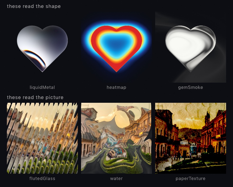
• .liquidMetal(repetition:softness:dispersion:distortion:contour:angle:tint:phase:) render the alpha shape as flowing chrome. Reflectance bands compress and wrap the silhouette as if the shape were inflated, and they carry chromatic fringing.
• .heatmap(colors:contour:innerGlow:outerGlow:angle:noise:phase:) thermal imaging of the alpha shape. Heat blooms inside, a halo radiates outside, and traveling waves pulse through. All of it is mapped cold to hot through colors, whose first stop fades to transparent.
• .gemSmoke(colors:body:innerSwirl:outerSwirl:innerGlow:outerGlow:offset:scale:angle:phase:) smoke coils trapped inside the alpha shape, and leaking around it, over a glassy body fill.
• .flutedGlass(flutes:shape:profile:distortion:shift:stretch:blur:edges:highlights:shadows:margins:angle:) ribbed architectural glass. Each flute refracts its slice of the image, and FluteProfile picks how (.prism / .lens / .contour / .cascade / .flat). FluteShape bends the flute layout (.lines / .irregular / .wave / .zigzag / .eggCrate). You also get boundary hairlines, shadow ramps, a frost blur, and margins in layer pixels, which leave a plain frame around the glass. The filter is static by design, so animate its parameters.
• .water(scale:waves:refraction:layering:edges:highlightAmount:highlightColor:phase:) the image under shallow rippling water. Broad waves wobble it, caustics shimmer it, and bright filaments wash over it.
• .paperTexture(paper:shading:contrast:roughness:fiber:crumples:folds:drops:seed:) lay the image onto a sheet of paper the filter synthesizes (tooth, fibers, crumple facets, fold creases, speckles), embossed by the same relief lighting. Static by design.
• .melt(colors:scale:warp:liquify:blend:phase:) the luminance melt. A warped noise field liquifies the layer, and the result is poured through a four-stop palette that runs dark to light. One displacement does two jobs. It warps the field's own domain and it shifts where the layer is sampled, so the picture smears along the field's currents while its brightness steers the field back. liquify is the smear, and blend is how much the image leads, where 1 reads the liquified picture straight through the palette. warp is the turbulence, and scale is the field zoom. The picture survives as light and shadow rather than as its own colors, and that dyed reading is the look.

let logo = makeRenderTarget()
withTarget(logo) { noStroke(); fill(.white); drawHeart(width / 2, height / 2, 400) }
drawImage(logo.filtered(.liquidMetal(phase: time)).image, 0, 0)

Filters chain, so an effect reads as one expression:

layer.filtered(.threshold(0.5)).filtered(.gaussianBlur(radius: 3)).filtered(.gradientMap(.magma))

combined(with:_:) and Combine

A Filter reads one layer, while a Combine reads two. It takes a base layer and an auxiliary layer that modulates it, which is what masking, displacement, and cross-dissolve need. base.combined(with: aux, op) runs the op on the GPU and hands back a new layer. That layer is filterable and combinable in turn, so multi-input effects chain like single-input ones.

A Combine is a value descriptor like Filter. A value descriptor cannot hold a RenderTarget, so the aux layer travels alongside it as the with: argument. A combine over a base that nothing drew into is skipped and its result stays empty, so draw the base first, if only a background(). The ops:

• .mask(channel:inverted:) keep the base where the aux reads bright (channel: .luminance, the default, so draw the mask in white over transparent) or opaque (channel: .alpha). Everywhere else the base fades to transparent, and inverted flips that. Use it for a spotlight reveal, a vignette, or a clip to a shape.
• .displace(amount:) offset the base's pixels by the aux read as a vector field. Red is horizontal, green is vertical, mid-gray is no shift, and the largest shift is amount of the layer. Feed it noise or a gradient for ripples, smearing, heat haze, and refraction.
• .disperse(amount:mode:spectral:quality:) chromatic aberration over the base, its amount scaled per pixel by the aux's brightness. A white aux splits by the full amount, and a black one leaves the base alone. So the aux decides where the color comes apart rather than how much. mode, spectral, and quality mean what they mean on .chromaticAberration.
• .mix(amount:) cross-dissolve the base toward the aux by amount (0 = base, 1 = aux). It is the everyday transition.
• .light(reach:brightness:bounces:sky:quality:) light a flat scene. The base is what light meets, and its alpha stops a ray. The aux is what gives light off, and the result is the light arriving at every pixel. One measurement gives you shadows that are sharp at the shape and soft further away, falloff, beams through a gap, and the color a lit wall gives back. The cost does not follow how much was drawn. See Light in a flat sketch and the Effects/Light example.
• .paintMix(amount:quality:) blend the base toward the aux the way scattering paints blend, rather than the way lights cross-dissolve. At each pixel both colors become reflectance spectra and mix through the Kubelka-Munk model, over a quality-sized set of wavelength taps. It is the GPU form of Color.mix(_:_:t:in: .paint) (see Spectral color). A yellow wash over a blue field meets it in green, and overlaps darken like glazes. The aux's own coverage gates the mix. Where the aux layer is empty the base passes through untouched, and the aux reads as paint laid over the base. amount is the mix where the aux is opaque.
• .seamlessClone(amount:threshold:) drop the aux layer into the base so the join disappears. The patch keeps its own detail and takes on the base's color and brightness, which is what stops a cut-out reading as a cut-out. It lands on the aux's opaque region, so draw the patch into a layer of its own, transparent everywhere else, positioned where you want it. Around the rim of the patch the op measures how far the patch's color sits from the base's. It spreads that difference across the inside as smoothly as it can, and adds it back. The rim then matches the base exactly, and the inside is nudged by the gentlest correction that reaches it. amount dials that correction: 1 is fully seamless, and 0 is a plain paste with the seam left in, which makes a useful before picture. threshold is the alpha a texel needs to count as part of the patch. Raise it if a soft-edged patch reads as larger than it looks. Two limits follow from what the op does rather than from how it is written. First, only the low, slow part of the patch's color is replaced, so the patch's range of tone is kept. Drop a contrasty patch somewhere much darker than itself and its shadows are pushed below black and clip. Second, the rim is where the whole answer comes from, so a rim laid across a hard edge in the base smears that edge inward. Keep the rim on quiet ground. See the Effects/SeamlessClone example.
• .lineIntegralConvolution(length:field:) brush the base along a direction field read from the aux. Every pixel becomes the average of the base along the streamline through it, walked both ways for length. That length is a fraction of the layer's long side, and it defaults to 0.04. Fine grain then comes out as streaks that follow the field, which is the classic way a flow is pictured. Give it a base with detail to drag, such as a .grain pass over a flat picture, a noise generator, or a photo. Pick how the aux is read with field. .vector (the default) takes red and green as a direction, with mid-gray meaning none, so a normal map or a hand-drawn flow steers it. .angle(turns:) reads the aux's brightness as a heading, black to white spanning turns full turns, so a noise layer turns into swirls. .contour runs the streaks along the level lines of the aux's brightness, around a blurred blob or along a gradient. Every field is unoriented, so a walk carries through where the field turns back on itself. A walk stops where the field is zero or at the layer's edge, so a flat aux hands the base back unchanged. One thing to know about .angle: at a hard edge between two tones the half-covered texel reads as the angle between them. That is a line along the edge, and a streak follows it instead of crossing it. Keep an angle field smooth, or harden its edges with .threshold first. The step count is capped, so a very long length walks in longer strides rather than more of them. See the Effects/FlowStreaks example.
• .defocus(focus:range:maxBlur:quality:) depth of field. It blurs the base by the aux read as a depth map, where luminance is the depth, 0 near and 1 far. The gray you draw is the depth the filter reads: Color(white: 0.47) means 0.47, whatever a linear-light layer stores it as, and a target's .depth layer is written so it reads back the same way, so a sketch never converts. The band focus ± range stays sharp, and the blur grows with distance from that band, reaching maxBlur pixels at the map's ends, 0 and 1, which for a scene's depth are the camera's near and far planes. The blur is the same gather depthOfField() runs on the canvas: each sample lands as a disc of light of its own size, and the samples in front of a pixel, at its own surface, and behind it are kept apart by distance. So a highlight keeps its light as it opens into a disc, a thin line in focus keeps its weight against a blurred background, a sharp subject keeps its edge, a defocused foreground covers what lies behind it by the share a lens gives, and a surface whose blur changes across it (a ball, a receding plane) spreads its light the way the lens does rather than by each sample's blur alone. The depth map can be a smooth gradient for a tilt-shift plane, a real depth feed, or hard-edged discrete per-object depths. All three work; a drawn map's anti-aliased rim is read as part of the nearer side, the way the canvas resolves a silhouette to its nearest surface. quality is a RenderQuality tier that sets the bokeh sample count, and the tiers are .default, .performance, and .detail, relative to the hardware. More taps trade frame rate for creamier, structure-free blur, so maxBlur is the blur amount and quality is the blur smoothness. Three parameters shape the highlights: blades, irisAngle, and catsEye. An out-of-focus point of light is a picture of the opening it came through. So an iris with blades makes that point a polygon of that many sides. A blades of 0 is round, and 5 to 11 is what a real lens carries. irisAngle turns the opening. The catsEye value (0 to 1) clips it toward the corners the way a lens barrel does. That lays a highlight down into a lemon shape the long way around the frame. The polygon is taken at the same area as the round opening. So a blade count changes the shape of a highlight, not how large it reads. catsEye changes shape only: a clipped opening carries the light a round one does, inside a blurred disc and past its silhouette alike, so use .vignette to darken the corners as well. Leave blades unnamed and it takes the blade count from the camera that drew the depth layer (Camera3D.apertureBlades). A 3D scene defocused by its own depth then uses the same opening its lens flare ghosts and its path-traced export do. Name it at the call to shape a blur no camera knows about, such as a tilt-shift over a hand-drawn ramp. The shape is as clean as the tap budget for most of the frame, and a median after the gather evens out the pattern the taps leave; a light much smaller than the spacing between taps is drawn as a disc of its own instead, scattered rather than gathered, so a point of light opens into an even disc at every quality. A round opening costs exactly what it always did, and a shaped one costs about a third more GPU time. See the Effects/Defocus example. To blur the main 3D canvas through the camera's own lens instead, use depthOfField().
• .ambientOcclusion(radius:amount:bias:quality:) ambient occlusion. It darkens the base in crevices, gaps, and where surfaces meet, reading the aux as a depth map. Ollin reconstructs the view-space position and surface normal from the depth, so there is no separate normal buffer. It then estimates occlusion with a hemisphere of samples oriented to the normal. The kernel is a dense low-discrepancy one, so it stays stable without per-pixel jitter. Ollin smooths the result with a depth-aware blur and multiplies it into the base. Feed it a 3D scene's own depth. That layer carries the camera's near and far planes and its field of view, so radius reads in world units. intensity scales the darkening. bias rejects self-occlusion, so raise it if flat faces speckle and lower it if contacts look weak. quality is the sample-count tier. As a post-process it darkens the final image rather than the ambient term alone. That is the standard screen-space trade, and intensity is how you dial it.
• .screenSpaceReflections(amount:maxDistance:thickness:roughness:fresnel:edgeFade:quality:) screen-space reflections. The scene reflects off its own surfaces, such as a glossy floor, wet asphalt, or a polished tabletop. The aux is read as a depth map. Each pixel's reflection ray is built from the view-space position and surface normal, then marched through the depth buffer until it meets the scene. The color found there is composited back over the surface. Feed it a 3D scene's own depth, because that layer carries the camera scale, so maxDistance reads in world units. intensity is the reflection strength. thickness is how close a ray must pass a surface to hit it. It is a fraction of the surface's distance, so it scales with the scene, and too large a value smears a reflection into a "cylinder". roughness blurs the reflection for a glossy rather than a mirror finish, and fresnel strengthens it at grazing angles. edgeFade fades a reflection as its ray nears the frame border, and quality is the ray-march step tier. It reflects only what is already on screen, so off-screen and hidden geometry cannot appear, and rays fade out as they reach the frame edge. Like all screen-space reflection, it is at its best on broad surfaces with well-separated reflected objects. A very dense scene, or one seen near grazing, can show faint artifacts where reflected surfaces graze the ray. A touch of roughness softens those, and the Examples/3D/Effects/ScreenSpaceReflections sketch shows a clean composition. Reflections are accumulated across frames, so they hold steady as the camera moves. The march runs at a resolution the quality tier sets, which is full on export. One limit is worth stating plainly. This effect makes a mirror out of the finished picture, and a picture does not contain the back of anything. Sometimes the true reflection is of a surface the camera cannot see. Examples are the underside of a ball resting on the floor, and the hidden face of a box. There the effect can only approximate, which shows as a soft, imperfect zone where objects meet the floor. For exact mirrors of real geometry, including hidden and off-screen surfaces, use rayTracedReflections() on a ray-tracing GPU. See Combining 3D features, which compares the two side by side.

let scene = makeRenderTarget()
withTarget(scene) { background(.black); fill(.orange); drawCircle(width / 2, height / 2, 300) }

let mask = makeRenderTarget()
withTarget(mask) { fill(.white); drawCircle(mouseX, mouseY, 200) }   // white = visible

drawImage(scene.combined(with: mask.filtered(.gaussianBlur(radius: 12)), .mask()).image, 0, 0)

The base and aux can render at different scales, because the aux is sampled by normalized coordinates. In a compose { } block the same ops read as aside modifiers (below). The Effects/Aside example shows a displacement map and a spotlight mask in one scene. Effects/PigmentMix runs .paintMix and .mix over one yellow-over-blue pair at once, one half by hand and the other through compose { }.

depth: a 3D scene's depth as a layer

The depth map .defocus reads can be one you draw by hand, but when the scene is 3D its depth comes for free. Draw a 3D scene into a render target. Because meshes or point clouds land in it, the target captures depth too, and target.depth exposes it. That is a gray layer (0 near … 1 far) the renderer fills from the scene's own depth buffer. Feed it straight to .defocus as the aux and a real 3D render racks focus like a lens, with no hand-drawn depth map needed. The same layer feeds .ambientOcclusion and .screenSpaceReflections. It carries the camera's near and far planes and its field of view, so their world-unit parameters (radius, maxDistance) read in the scene's own scale.

let scene = makeRenderTarget()
withTarget(scene) {
    perspective(eye: Vector3(0, 2, 18), target: .zero, near: 5, far: 34)   // bracket the scene
    drawSphere(radius: 1.5)                                                 // 3D → depth captured
    // … more meshes …
}
let dof = scene.combined(with: scene.depth, .defocus(focus: 0.4, maxBlur: 30))
drawImage(dof.image, 0, 0)

scene.depth maps over the camera's near and far, so set them to bracket your scene. Tight planes make the focal plane sweep usefully, and they give the depth buffer its best precision. The gray runs evenly with distance (a point halfway between the two planes reads 0.5, whatever curve the depth buffer itself stores), and it measures depth along the camera's view axis rather than distance from the eye. So a world point p sits at ((p - eye).dot((target - eye).normalized) - near) / (far - near), which is the focus that puts the focal plane on it. depth(at:) answers in clip space, for placing 2D marks among 3D ones, so it is not that number. It is a normal layer otherwise, so draw it with drawImage(scene.depth.image, 0, 0) to see the depth, or filter it. Depth capture costs nothing on a 2D target, because no 3D drawn means no depth buffer. The extra normalize pass runs only when you read .depth. The SceneDefocus example racks focus through a row of orbs by their own depth.

generate(_:) and Generator

A Generator is a procedural pattern filled from math alone, with no input layer. Where a Filter transforms a layer you drew, a Generator is a layer. It is a source you composite, filter, or feed into another effect. generate(_:) turns one into a RenderTarget, which is drawable and filterable, so a pattern flows straight into the rest of the chain. The Effects/GeneratorCatalog example shows the basic patterns, the design set, and the composed chains, and Effects/MeshGradient shows the mesh gradient.

let stripes = generate(.bars(scale: 24, foreground: .black, background: .white))
drawImage(stripes.filtered(.gaussianBlur(radius: 4)).image, 0, 0)

// A layered mix: noise → colormap, with a grid multiplied over it.
let field = generate(.noise(scale: 5)).filtered(.gradientMap(.turbo))
drawImage(field.image, 0, 0)
blendMode(.multiply)
drawImage(generate(.gridLines(scale: 20, weight: 0.08)).image, 0, 0)

The basic patterns (cells stay square whatever the layer's aspect ratio):

• .checkers(scale:foreground:background:) a two-color board, scale cells across.
• .gridLines(scale:weight:foreground:background:) a line grid, each line weight (0…1) of a cell wide.
• .bars(scale:vertical:foreground:background:) parallel stripes, scale across, on either axis.
• .noise(scale:sharpness:warp:foreground:background:) fractal value noise, running from a soft cloud (sharpness 0) to a hard two-tone split (1). The warp value domain-warps the field, meaning the layers displace their own sampling coordinates, twice over. A warp of 0 is the plain field, and 1 is the classic flowing marble-and-cloud smear.
• .cellular(scale:jitter:style:foreground:background:phase:) Worley cellular noise, scale cells across. style is .cells (dark cores brightening toward the walls), .borders (thin cracks tracing the walls), or .mosaic (flat stained-glass panes). jitter runs the cells from a regular grid (0) to fully organic (1). phase makes the feature points wander on small orbits, so the cells crawl and reform. It is periodic over 2π, so phase: loopProgress(over: 12) * .tau loops seamlessly. See the Cellular example.
• .gaborNoise(wavelength:bandwidth:angle:spread:impulses:phase:seed:foreground:background:) Gabor noise, a field whose spectrum you design instead of inherit. Every kernel is a small Gaussian blob carrying a cosine wave, scattered at random and summed, so the field has one principal wavelength (in pixels) and, when spread is small, one direction: brushed metal, wood grain, straw, silk. bandwidth is the width of the band around that wavelength as a fraction of it, where 0.2 is nearly a pure wave with long interference patterns and 1 is blobby. angle is the wave direction (0 oscillates along x, so the stripes stand vertical), and spread is how far each kernel's own direction may wander from it: 0 is one direction, π (the default) every direction. impulses is how many kernels overlap at any point, the quality dial. phase slides every wave along its own direction and is periodic over 2π, so phase: loopProgress(over: 8) * .tau loops. A field at angle + .pi is the same field, so angle: loopProgress(over: 8) * .pi loops too. The kernels are filtered for a one-pixel footprint, so a wavelength driven toward two pixels fades to gray instead of aliasing. The CPU gaborNoise computes the same field at the same pixel. See the GaborNoise example.

Design patterns: richer animated sources in the same mold. Every one takes a phase you feed time for motion, or hold fixed for a still. Most take a palette of colors plus a background, and a centered composition stays centered and round at any canvas aspect. Their palettes blend in sRGB, the space design gradients are authored in, so the mixes match what a design tool would show:

// An animated wallpaper in one call.
drawImage(generate(.meshGradient(phase: time)).image, 0, 0)

• .meshGradient(colors:distortion:swirl:mixing:grain:phase:) soft blobs of up to 8 colors drifting on orbits, blended into the classic mesh-gradient wash. distortion smears it organically, and swirl winds a vortex. mixing runs the blend from hard poster cells (0) through the classic look (0.5) to a smooth wash (1), and grain dithers the boundaries and films the result.
• .filaments(color:highlight:background:scale:brightness:contrast:phase:) a glowing web of thin writhing filaments, the neural-lace look.
• .smokeRing(colors:background:radius:thickness:fill:scale:detail:phase:) a billowing ring of smoke, radially banded through the palette, and fill softens it from crisp ring toward a smoky disk.
• .colorPanels(colors:background:density:length:skew:blur:fadeIn:fadeOut:gradient:phase:) translucent color panes fanning around a central axis in fake perspective.
• .spiral(foreground:background:density:distortion:strokeWidth:taper:cap:noise:noiseScale:softness:scale:phase:) a two-color spiral, from crisp line-art through whirlpool to wobbly hand-drawn rings.
• .waves(foreground:background:shape:frequency:amplitude:spacing:proportion:softness:scale:phase:) wavy-line stripes, where shape (0…3) morphs zigzag → sine → irregular mixes.
• .dotOrbit(colors:background:scale:size:sizeVariation:spread:steps:phase:) a grid of dots, each orbiting its own cell on its own phase, colors quantized to flat print-like shades.
• .grainGradient(colors:background:shape:softness:amount:noise:phase:) poster-style banded gradients over an animated field (GrainShape: .wave / .dots / .truchet / .corners / .ripple / .blob / .sphere), the band edges chewed by film grain.
• .pulsingBorder(colors:background:roundness:thickness:softness:amount:bloom:spots:spotSize:pulse:smoke:smokeScale:margins:phase:) a glowing rounded border hugging the layer edge (inset by margins, in layer pixels), up to eight light spots per color racing the perimeter, with a heartbeat pulse and smoke wisps.
• .godRays(colors:background:center:density:breakup:coreSize:coreIntensity:intensity:bloom:bloomTint:phase:) crepuscular rays streaming from a point, one drifting streak layer per color. bloom morphs the stack from alpha layering to additive light, and bloomTint washes an extra glow color over the lit areas.

Pattern fields: closed-form animated fields, each a few lines of per-pixel math with a look of its own. They follow the same conventions as the design patterns, with a phase to feed time, sRGB palette blending, and square cells at any aspect:

• .quasicrystal(colors:background:symmetry:scale:contrast:phase:) plane waves at symmetry evenly spaced angles, summed into a pattern that is ordered but never repeats, with crisp N-fold stars around its bright centers. The field walks the palette, contrast sharpens the walk, and phase shimmers the whole crystal.
• .moire(foreground:background:sources:frequency:scale:phase:) a few concentric ring gratings on slowly orbiting centers, and where they overlap, their beat sweeps out large fringes that move much faster than the centers do.
• .gyroid(foreground:background:scale:thickness:phase:) a planar slice of the gyroid surface, drawn as interwoven organic bands with a dimmed echo for depth, and phase sweeps the slicing plane so the bands crawl and reconnect.
• .phyllotaxis(colors:background:count:dotSize:phase:) the sunflower's seed arrangement (golden-angle spiral) as a continuous dot field, colored center-to-rim by age. Past dotSize ≈ 1 the dots fuse into a cellular texture, and phase spins the head.
• .hexPulse(colors:background:scale:gap:phase:) a hexagonal lattice whose every cell breathes on its own hashed rhythm, brightness and a little size following the pulse.
• .chladni(m:n:style:weight:grain:foreground:background:scale:phase:) the standing-wave field of a ringing square plate. .sand gathers speckled ink along the still nodal lines, where weight is the gather width and grain runs from smooth ink to loose sand, shivering as phase advances. .wave breathes the signed field between the colors. Integer m and n ring true modes, and fractional values morph between figures. The full story, covering the CPU field, nodal isolines, and the audio join, is on its own page.

See Examples/Effects/GeneratorCatalog for the fields family, whose chains family has the field chained into .relight, and Examples/Patterns/Chladni for the plate.

Escape-time fractals: the classic sets as generators, colored by the smooth, stepless iteration count through the palette, with phase cycling the bands:

• .mandelbrot(colors:interior:center:zoom:iterations:cycles:phase:) the Mandelbrot set. It iterates z = z² + c from zero at every pixel's c and colors by how fast the orbit escapes. Points that never escape are the set, painted interior. center and zoom frame the complex plane the way every generator on this page does. center sits in the middle of the picture, 3 / zoom units run across its shorter side, and the imaginary axis points up. Zoom 1 shows the whole set, and float precision holds useful detail to a few thousand times in. iterations caps the orbit, so raise it as you zoom.
• .julia(c:colors:interior:center:zoom:iterations:cycles:phase:) a Julia set. It is the same iteration with c fixed and the orbit started at each pixel, so every c yields a different filigree, and points near the Mandelbrot set's edge give the richest. Animate c a little and the whole form morphs.
• .orbitTrap(_:c:colors:center:zoom:iterations:glow:angle:) an orbit trap. It runs the same iteration, but colors by the orbit's closest pass to a trap shape held in the plane rather than by its escape. Orbits that graze the trap glow through the last of colors, and distant ones sit in the first. Stalks and filaments appear wherever orbits pass near the shape. The trap is a Generator.OrbitTrap: .point(_:), .cross(_:) for the stalk look, .circle(center:radius:), or .square(center:radius:), with the outlines lit from both sides. c: nil works the Mandelbrot plane, and a fixed c picks that Julia set and re-centers the default framing. glow is the falloff distance in plane units, so tighten it to thin the filaments. angle turns the trap about its own center, so feed it your time and the stalks sweep.

Each of these, and the domain coloring and Newton's basins below, hands its framing back as a ComplexPlane through plane. With it a sketch marks a number on the picture, or reads the number under the pointer, without redoing the arithmetic. canvasPoint(of:in:) says where a number lands in the rectangle the picture was drawn in. planePoint(at:in:) reads the number under a canvas point:

let julia = Generator.julia(c: Vector2(-0.79, 0.15), zoom: 1.2)
drawImage(generate(julia).image, 0, 0)
if let plane = julia.plane {
    let z = plane.planePoint(at: mouse, in: bounds)                    // the number under the pointer
    drawCircle(center: plane.canvasPoint(of: .zero, in: bounds), radius: 6)   // the origin, marked
}

The Complex page has the framing in full.

Newton's basins: the same plane, asked where an orbit ends up rather than when it left. .newton runs Newton's method, z -= p(z) / p'(z), from every pixel over the polynomial whose roots you place. Each pixel takes the color of the root it lands on, so every root owns a basin. Wherever two basins meet every other one is there too, at every scale, so the boundaries are dust where all the colors touch:

• .newton(roots:colors:trapped:shading:relaxation:center:zoom:iterations:phase:) up to eight roots on the plane (the default is the three cube roots of one). The palette is spread around the roots in order, so pass one color per root for exact control, and phase turns it around the wheel without recomputing anything. shading (0…1) darkens a pixel by the steps it took, bright at the root and dark toward the edge, with a faint contour per step. A pixel the method never brings to a root within iterations is painted trapped: rare for a plain polynomial (z³ - 2z + 2 has a cycle at 0 and 1 that catches it), common once relaxation leaves 1. That dial scales the step: 0.6 creeps and the basins fatten, 1.4 overshoots and they spiral and shed islands, and past 2 nothing lands. center and zoom frame the plane as every generator here does: center in the middle, 3 / zoom units across the shorter side, the imaginary axis up.

See Examples/Effects/NewtonBasins, where the roots move on slow orbits and the step's scale is a dial.

Diffusion: not a look laid over a picture, but a picture made out of a few marks. .diffuse holds every drawn pixel as a color source and lets the color out into the empty space between them until it settles. Away from the marks every pixel ends up the average of its four neighbors, which is the rule a soap film obeys. So the field is smooth everywhere, nothing overshoots, and no color appears that was not put there. In the math it is a Laplace solve, the fill also called harmonic, membrane, or Poisson interpolation. It is not poissonDisk, which scatters points.

• .diffuse(threshold:sharpness:) a pixel counts as a source when its alpha is at least threshold, and a half-opaque mark pulls half as hard as a solid one. So draw the marks into a layer of their own and filter that. sharpness (0…1) decides how far the solve is pushed, from three rounds at 0 to six at 1. Each round takes about half of the error left in the far field, so three leave a few percent and six leave nothing a level can measure.
• drawDiffusionCurve(_:left:right:width:) lay down the form the technique is named for. It draws the same path twice, a hair apart, carrying a different color on each side, so the field jumps across the curve and is smooth everywhere else. Left and right are named from walking the path in the order its points come, so reversing them swaps the colors. It takes a Contour or bare points, and width is how thick each side's mark is, where two or three points is plenty.

let marks = makeRenderTarget()
withTarget(marks) {
    drawDiffusionCurve(horizon, left: Color(hex: 0xE86F4A), right: Color(hex: 0x101A2E))
    noStroke(); fill(Color(hex: 0xFFE9B0))
    drawCircle(width * 0.7, height * 0.2, 26)     // a light the whole field bends around
}
drawImage(marks.filtered(.diffuse()).image, 0, 0)

A gradient needs a direction and two ends. This needs neither, which is why the field can be shaped by where the marks are rather than by a line between two stops. See Examples/Effects/DiffusionCurves.

The fill takes its colors from the sources' edges, so what sits at the edge of a mark is what spreads. That matters when the sources are cut out of something soft. Marks keyed out of a glow with .lumaKey(low:) have rims at about the key level by construction, since the key is where they begin, and the field comes out near that level too, dim, however bright the centers are. Key one layer for where the sources are, and take their color from a second layer drawn at full strength, masked by that key, so the edges carry the color you meant:

let key = glow.filtered(.lumaKey(low: 0.3))                    // where the sources are
let sources = paint.combined(with: key, .mask(channel: .alpha)) // what color they are
drawImage(sources.filtered(.diffuse()).image, 0, 0)

The solve is the frame's cost, about 24 ms of GPU at 1080 square on an M2, and it runs every frame while the marks move. When they do not move, solve once instead. Hold the filtered layer in a property, fill it in setup(), and draw it each frame like any other image.

Measured distance fields: a question asked of a layer rather than a look laid over it. .distanceField measures how far every pixel is from the nearest edge of whatever was drawn, and which way that edge lies. .fieldMap reads the answer back as a picture. Growing and shrinking a shape, outlining it at an offset, drawing its contour lines, and building a Voronoi keyed to the marks themselves are all one small step from there.

• .distanceField(from:threshold:maxDistance:) measure the field. Red is the distance in pixels, negative inside the shape. Green and blue are the unit direction to that nearest edge, so pixel + direction * abs(distance) is the edge point itself. from chooses what the threshold cuts, which is .alpha by default, or brightness or one channel for a layer with no transparency in it. maxDistance both bounds the answer and shortens the work.
• .fieldMap(_:from:to:repeating:) read a measured field back through a Ramp or Colormap, over a window given in pixels. With repeating the window wraps rather than clamps, which draws the field as contour bands.

let field = marks.filtered(.distanceField())
drawImage(field.filtered(.fieldMap(.viridis, from: 0, to: 40, repeating: true)).image, 0, 0)

A user shader reads the field with sampleRaw, which returns the layer's stored values with no color conversion, and that is how the direction gets used. The whole surface, including the nearest-edge shader, is in Measured distance fields. See Examples/Effects/DistanceField.

The measurement costs about 4.9 ms of GPU at 1080 square on an M2 over the whole canvas, and about 2.9 ms capped at 64 pixels.

Domain coloring: the same plane, asked a different question. Instead of iterating, it evaluates a complex function once at every pixel and paints the direction its answer points, off a palette wheel that wraps. The last stop blends back into the first, so a turn has no seam. What you get is readable. A zero shows the whole wheel once turning counter-clockwise, a pole shows it once the other way, and a repeated zero shows it twice. Counting wheels counts zeros and poles, which is the argument principle drawn rather than proved.

• .domainColoring(_:colors:shading:strength:center:zoom:phase:) the function is a Generator.ComplexFunction. .rational(zeros:poles:) places up to four of each and is the one to move around, so repeat a point for a double zero, and leave poles empty for a polynomial. .power(_:) winds the wheel that many times, and a fractional exponent leaves the seam of its branch cut on show. .exponential, .sine, and .tangent are the classics, with tan z alternating zeros and poles along the real axis. .logarithm draws its own cut down the negative real axis.
• shading is a Generator.DomainShading. .phase is color alone, the plain phase portrait, with every point fully lit. .modulus ramps dark to light between each doubling of the value's size, which is a contour map of magnitude. .conformal rules direction too, twelve sectors to the turn, so away from the interesting points the field tiles into little squares. strength (0…1) sets how hard the rulings press.
• center and zoom frame the plane as they do for the fractals: center in the middle of the picture and 3 / zoom units across its shorter side, so zoom 1 shows 3 units. The imaginary axis runs up the canvas, as it is written on paper. plane hands the framing back as a ComplexPlane, for placing a zero on the picture. phase turns the palette around the wheel and only recolors, so phase: time * 0.05 is free.

See Examples/Effects/DomainColoring for the four above, one of them swimming its zeros.

See Examples/Effects/EscapeTime for the first two, with the Julia's c on a slow orbit, plus all four traps, two of them turning.

A pattern composes for the layer it fills. The default generate(_:) makes a full-canvas layer, and generate(_:width:height:) fills one of an explicit size, so a tile or panel gets its own undistorted pattern instead of a squashed full-canvas one.

postProcess(_:)

Apply a filter to the whole finished frame, just before it is shown. It is the quick way to bloom or blur everything without managing a layer:

override func draw() {
    background(.black)
    // …draw a bright scene…
    postProcess(.bloom(threshold: 0.7, amount: 1.2))   // glow the whole frame
}

Call it in draw(), and multiple calls chain in order.

withOverlay(_:)

Draw over the finished frame. Everything in the block is held back and drawn after the frame's own passes: the temporal anti-aliasing, the depth of field, the motion blur, the lens flare, and the postProcess filters. A caption, a frame, or a readout drawn here stays sharp and untinted whatever the scene under it does:

override func draw() {
    background(.black)
    var lens = Camera3D.perspective(eye: Vector3(0, 1, 5), target: .zero)
    lens.aperture = 0.12         // a lens with an opening blurs by depth
    camera(lens)
    depthOfField()
    drawMesh(Mesh.sphere(radius: 0.6))   // the scene, blurred by its depth
    withOverlay {
        fill(.white)
        drawText("f/1.4", 24, height - 24)   // sharp over the blurred scene
    }
}

Everything in the block lands above everything outside it, in the block's own call order, however the calls were interleaved. It is scoped like withState: drawing state and transforms carry in, and any change is restored on exit. A blend mode in the block blends against the finished frame, so a .multiply darkens the picture under it. A withClip inside clips the overlay alone. The overlay carries its own depth, cleared, so a 3D shape drawn here sorts against the others in the block and sits over the scene without joining its shadows or its lens. Over the accumulation surface of noClear() the overlay is drawn over the pile each frame and never joins it, which is how a readout sits over a drawing that keeps piling up. Inside a withTarget block it draws into the layer, since a layer has no passes to draw after. A vector export writes it after everything else.

makeFeedback(scale:) and withFeedback(_:_:)

A Feedback layer remembers itself across frames. Each frame you read last frame's content, transform it by fading, zooming, rotating, or offsetting it, and draw new content on top. The result becomes next frame's content. That read, transform, and write loop is what makes trails, tunnels, and the video-feedback look of a camera pointed at its own screen.

This is not the same as the accumulation surface (noClear), which piles new draws onto an unchanging canvas. Feedback hands you the previous frame as an image you can transform before drawing it back, and that transform step is the whole effect.

makeRenderTarget() gives you a per-frame handle, but a Feedback is persistent, so make it once in setup() and hold it. Its identity is what ties this frame's write to last frame's read. Make a fresh one each draw() and nothing ever builds up.

var trail: Feedback!

override func setup() { trail = makeFeedback() }      // make once, store it

override func draw() {
    background(.black)                            // clears the canvas (resets the frame)
    withFeedback(trail) { prev in                 // prev = last frame's content
        translate(width / 2, height / 2)          // spin + shrink the old frame
        rotate(0.06); scale(0.98)                 //   about the canvas center
        translate(-width / 2, -height / 2)
        tint(Color(white: 1, alpha: 0.94))        // gentle decay so trails fade
        drawImage(prev, 0, 0)
        noTint()
        fill(.white); drawCircle(mouseX, mouseY, 12)   // a fresh mark on top
    }
    drawImage(trail.image, 0, 0)                  // composite the result to the canvas
}

• withFeedback(_:_:) hands the previous frame in as the closure parameter. The withTarget(feedback) { … } form works too, reading last frame by name with feedback.previous inside.
• feedback.previous is last frame's content, and feedback.image is this frame's, for compositing.
• feedback.filtered(_:) runs this frame's result through a Filter like any layer, so you can bloom the trails or recolor them through a gradient map. feedback.combined(with:_:) makes it the base of a Combine, so the trails can be masked, displaced, or mixed by another layer. The state the loop carries forward stays untouched either way. An Accumulator and a SimField take both calls too.
• makeFeedback(precision: .float32) keeps the pair in single-precision float, for a loop that carries a long sum of faint light. Half float stops moving once each frame's contribution falls under one part in a thousand of the total. For a sum that should converge rather than grow, an Accumulator keeps the sum in single precision and divides by the passes for you.
• Inside the block, background(_:) clears the feedback layer alone. The canvas's own background(_:), before the block or after it, leaves the layer as it was.
• See the Effects/Feedback example for a spiralling tunnel.

makeSimField(_:) and Sim

Where a Filter transforms an image once, a Sim runs a stateful simulation on a persistent layer. The layer evolves every frame by reading its own neighborhood: reaction-diffusion patterns spreading, cellular-automaton cells living and dying, a fluid carrying color. Pick a Sim from the catalog, make a SimField with it, and draw into the field to seed or force it. When the catalog has no rule for you, write the kernel yourself and the field runs it the same way.

A SimField is persistent like Feedback, so make it once in setup() and hold it. Each frame the marks you draw in withField land on the field's current state. The renderer then steps the simulation, and the result is the field's image. The raw state is data, so recolor it through the same Filter catalog as everything else.

var rd: SimField!

override func setup() { rd = makeSimField(.reactionDiffusion(), scale: 0.5) }   // half-res field

override func draw() {
    withField(rd) {                                  // draw to seed: marks inject chemical
        noStroke(); fill(.white)
        if mouseIsPressed { drawCircle(mouseX, mouseY, 16) }
    }
    drawImage(rd.filtered(.gradientMap(.magma)).image, 0, 0)   // evolve, then recolor
}

The catalog:

• .reactionDiffusion(feed:kill:) Gray-Scott reaction-diffusion, where two chemicals diffuse and react into coral, spots, stripes, and dividing cells. Draw light marks to inject chemical B, which spreads from there, and feed and kill pick the regime. The state is A in red and B in green. Recolor it with .gradientMap or .threshold. The .reactionDiffusion(feed:kill:toFeed:toKill:) form lets the regime vary across the field. Set the field's modulation to a layer. Its brightness then slides feed and kill per texel. The slide runs from the first pair where the map is black to the to pair where it is white. It stays one continuous simulation, so the pattern flows across the regime boundary instead of seaming at it. Use a camera matte as the map and it grows maze walls on a silhouette and spots everywhere else, which is the Vision/TuringMirror example. Any drawn or generated layer steers it the same way. Draw the map each frame before reading the field, because a frame with no map runs the plain black-end pair.
• .predatorPrey(halfSaturation:predatorGrowth:predatorDeath:steps:) two populations on one land, the Lotka-Volterra idea in the form Rosenzweig and MacArthur gave it. Prey breed toward the land's capacity. Predators eat them at a rate that saturates when prey are plentiful, then die off at their own rate. Both wander by diffusion. The field rests at full prey and no predators, so draw green to release predators. A mark's red sets the prey level and its green the predator level, both read in linear light like every sim's marks, and a black mark clears both. Where predators land on full prey the two chase each other around a cycle. Neighbors run a little behind each other, so the cycle becomes waves: an invasion front, then spiral waves curling through its wake. The defaults sit past the model's oscillation threshold, the regime that makes spirals. Raise halfSaturation toward 1, or predatorDeath toward predatorGrowth, and the cycle calms into a steady coexistence and the waves die out. steps is the pace, integration steps a frame. The raw image reads prey in red and predators in green, already a picture. A .gradientMap reads the mix by brightness, so one ramp paints bare soil, meadow, and the predators' color in turn. Wave size follows the field scale. See the Simulation/PredatorPrey example.
• .gameOfLife() Conway's Game of Life (B3/S23). Draw white to make cells alive, black to kill them. Use a low field scale so each texel is a visible cell. The image is crisp black-and-white.
• .lenia(radius:growthCenter:growthWidth:timeScale:rings:) Lenia, the continuous Game of Life. The state is a smooth 0...1 mass. Each step convolves it with a soft ring kernel. It then grows or starves every texel by how close its neighborhood mass sits to growthCenter. The growthWidth value is how forgiving that rule is. Blobs pulse, split, and swim. Seed it with a dense soup of soft gray-to-white marks, because sparse mass starves. The dying, labyrinth, rings, and fat-maze looks are all real regimes of the model, so if everything fades, seed denser or widen the growth. The kernel reads radius texels around every texel each step, which makes the field scale the cost lever. SimField.sim is settable live (field.sim = .lenia(...)), so growth settings can come from a @Param. The image is grayscale mass, so recolor it with .gradientMap. The CPU cellular automata (Wolfram rules, turmites) live in Generators → Cellular automata.
• .smoothLife(radius:birth:survival:intervalSoftness:cellSoftness:) SmoothLife, Rafler's generalization of the Game of Life to a continuous field, the rule the smooth glider lives in. A cell is a disc rather than a texel, and its neighborhood is the ring around it out to radius, with the ring three times the disc's width. Each step reads how full the disc is and how full the ring is. Life's birth and survival counts become two intervals of ring filling. A dead cell is born when its ring's filling lands in birth, and a live one survives when it lands in survival. The edges of those intervals are soft steps, intervalSoftness wide, and cellSoftness is how gradually a half-full disc counts as alive. The defaults are the paper's glider regime: blobs that hold their shape and slide in any direction, rings that pulse, colonies that split. Draw white to add living matter. The classic glider seed is a disc a little under the radius with a notch bitten out of one side, and black erases. Each step reads every texel within radius, so the field scale is the cost lever. A glider is about two radii across, so scale also sets its size on the canvas. The image is grayscale life, made for .gradientMap. See the Simulation/Automata example (its smooth rule).
• .ripples(speed:damping:) a water surface, running the 2D wave equation on a height field, the classic interactive ripple pool. A drawn mark's brightness is added to the surface height, and this sim's inject leaves the velocity channel alone. The bump then collapses, and rings spread, reflect softly off an absorbing rim, and die away by damping. Dab soft marks and do not hold them, because an opaque held mark pours water every frame. A drawCircle under a radial gradient fading to clear is the ideal drop. A hard-edged disc rings at every frequency, which is a real splash. The state is height in red and velocity in green, both signed. The raw image is a debugging view, so recolor it, or shade it as a surface with .filtered(.relight(...)). speed is the neighbor-coupling gain and is capped at 1. The step goes unstable at 2. There the shortest wave the grid can hold grows with every step, and settles into a grid-scale rattle that shades into glitter. Rings still travel at a good pace, because the step takes six substeps a frame. See the Simulation/Ripples example.
• .multiScaleTuring(scales:seed:) McCabe's multi-scale Turing patterns: one substance, looked at through several magnifications at once. Each scale averages the field over a small disc, the activator, and a larger one, the inhibitor. Where the small average is the greater the field brightens a little, and otherwise it darkens. That rule at a single scale grows the stripes of a zebra. At several scales, each pixel each step runs them all and lets only the one whose two averages disagree least act. So broad forms and fine detail settle into the same picture, and it comes out looking like an electron micrograph of a diatom. Unlike the rest of the catalog, a Turing field needs no seeding. It starts from noise and organizes itself, so reading it is enough to run it. A withField block is only for disturbing a settled pattern, where a mark's brightness replaces the field and the pattern heals around it. Edges wrap, so the picture tiles. The image is grayscale, ready for .gradientMap, or for .relight to read it as relief. Try the relief first, because the lit-from-above look is an accident of a flat 2D rule and reads as real depth. See the Simulation/MultiScaleTuring example.
• .cyclic(states:threshold:range:neighborhood:seed:) Griffeath's cyclic cellular automaton. Every cell takes one of states colors arranged in a circle. A cell advances to the next color the moment at least threshold neighbors already have it. So each color eats the one before it and is eaten by the one after. The field needs no seeding. It starts from seeded random states, because a uniform field is a fixed point and noise is the required start. The same seed replays the same run. From there it self-organizes through the famous four acts: colored static, growing droplets, spiral defects, and finally a field of turning spiral cores. The defaults are the classic rule, with 14 states, threshold 1, and CellNeighborhood.vonNeumann, the four edge-sharing neighbors. Raising threshold with a wider range (and .moore, the eight-cell block) trades spirals for churning block turbulence. Drawing stamps states, where brightness picks the state and white is the top, and the flow swallows the wound. The image is one flat gray level per state. It is made for .gradientMap with a ramp whose last stop repeats the first hue, so the wheel closes without a seam. One texel is one cell, and edges wrap. See the Simulation/Automata example (its cyclic rule).
• .excitable(states:threshold:range:neighborhood:) the Greenberg-Hastings model, the classic cellular automaton of excitable media such as heart tissue, neurons, and a chemical oscillator. A resting cell fires when at least threshold neighbors are firing, then climbs alone through its refractory tail back to rest. Mid-recovery it cannot be re-lit, which is exactly what turns a spark into a traveling ring with a dead zone behind it. Rings annihilate where they collide, and a broken front curls into a pair of counter-rotating spirals that re-excite the medium forever. The field starts at rest, so draw to spark it. A bright mark excites the cells it covers, and a black mark calms them. Dab sparks for rings, or excite a line, let it grow, then wipe half the plane with black, and the cut ends curl into spirals. Rest reads black, a firing cell faint gray, and the refractory tail climbs toward white. Run it through .gradientMap with a dark-to-hot ramp so the wavefronts glow. See the Simulation/Automata example (its excitable rule).
• .briansBrain() Silverman's three-state automaton, where every cell is ready, firing, or resting. A ready cell fires on exactly two firing neighbors. A firing cell spends the next step resting and cannot be re-lit, and a resting cell returns to ready. Almost nothing settles, so the field boils forever, with gliders racing along diagonals and orthogonals. So draw loose sprinkles, not solid blobs. A solid blob dies at once, because every interior cell rests together and a flat edge shows three neighbors where a birth needs exactly two. A random soup explodes into permanent traffic instead. The raw image is already the classic picture (white fire, mid-gray afterglow, black ground), and a .gradientMap restyles it. See the Simulation/Automata example (its brain rule).
• .forestFire(growth:lightning:neighborhood:) the Drossel-Schwabl forest fire, the automaton that made self-organized criticality visible. Every cell is empty, a tree, or burning. A burning cell is empty next step. A tree catches from any burning neighbor, and otherwise catches on its own with probability lightning. An empty cell grows a tree with probability growth. Nothing in the rule aims at a density, and one arrives anyway: trees fill in until a stand is connected enough for a strike to run through it, the fire clears exactly that crowd, and the field hovers there forever, throwing fires of every size from a single tree to most of the map. Keep lightning far below growth, because the ratio between them is what sets how big fires get, and a rate near growth burns every tree as soon as it grows. The field needs no seeding: it starts bare and grows itself in. The coin each cell throws is a hash of the cell and the field's own frame count, so a run replays exactly. Drawing stamps states, where white sets cells burning, mid-gray plants trees, and black clears a firebreak the flames cannot cross. A mark lays the nearest of the three, and its soft rim writes nothing. Two rims beside one gap do add up to a mark, though. So plant a dense stand by its outline, a percolation's outlines(of:in:) filled as a Shape, rather than a rect a cell. The raw image is grayscale (bare black, trees mid, fire white), made for .gradientMap with a ramp running dark ground to green to hot. .moore spreads fire through diagonal gaps and reads rounder than the classic four. One texel is one cell, and edges wrap. See the Simulation/Automata example (its forest rule).
• .hodgepodge(states:infectedDivisor:illDivisor:infectionRate:neighborhood:seed:) the Gerhardt-Schuster hodgepodge machine, the automaton built to mimic an oscillating chemical reaction. Its curling wavefronts are dead ringers for the Belousov-Zhabotinsky reaction in a dish. Cells run from healthy (0) through degrees of infection to ill (states). A healthy cell catches ⌊a/infectedDivisor⌋ + ⌊b/illDivisor⌋ from its infected and ill neighbors. An infected cell climbs to its neighborhood's average infection plus infectionRate. That is the speed of infection and the behavior dial: low dies out, mid plateaus, and high locks into the spiral regime. An ill cell recovers to healthy at once. Like the cyclic automaton it needs no seeding, because all-healthy is a fixed point. It starts from seeded random states, and the same seed replays the same run. Drawing stamps degrees of infection, and the waves close over the wound. The image is the infection degree as grayscale, made for .gradientMap across a hot or rainbow ramp, the classic way these figures are pictured. See the Simulation/Automata example (its hodgepodge rule).
• .wireworld() Silverman's Wireworld, the automaton that computes. Every cell is empty, a conductor, an electron head, or an electron tail. A head becomes a tail, a tail becomes conductor, and a conductor becomes a head when exactly one or two of its eight neighbors are heads. That last clause is the whole machine. One or two lets a signal run down a wire (the tail behind it cannot be re-lit, so it never runs back) and split at a fork, and three or more stops it, which is what a diode and every gate are built from. A loop of wire with one electron on it is a clock, a wire tapped off the loop carries its pulses, and two wires that join make an OR. The field starts empty, so draw the circuit. A mark's brightness picks what it lays down, snapped to the nearest of the four states: black erases, a third gray is conductor, two thirds a tail, and white an electron head. WireworldCell names those levels (.empty, .conductor, .head, .tail), so a sketch writes fill(WireworldCell.conductor.color) and .head.color, and the usual way in is a circuit typed as a few lines of text, one character per cell, stamped with drawRect on the first frame. Make the cells large enough to read (a low field scale), because a circuit is a picture of its wiring. The raw image reads back the same four levels, made for .gradientMap with a color per state, and the classic picture is yellow wire with blue heads and red tails on black. The eight-cell neighborhood lets an electron cut a ring's corners, so a nine-by-five ring is a clock with a period of twenty. Edges wrap. See the Simulation/Automata example (its wire rule).
• .schelling(preference:vacancy:mobility:passes:seed:) Schelling's model of segregation, the board that showed how a mild preference sorts a neighborhood. Every cell is empty or holds an agent of one of two kinds. An agent is content when at least preference of its occupied neighbors are its own kind, and one that is not moves to an empty cell nearby, taking a cell where it would be content when there is one within reach and stepping toward one otherwise. Nobody on the board wants to live apart, and it sorts itself into patches anyway, more sharply than anyone on it asked for. That gap between what each agent wants and what all of them get is the result the model is famous for. The field needs no seeding. It starts as a seeded random mix of the two kinds with vacancy of the cells empty, because a sorted board is a fixed point, and the same seed replays the same run. The empties are where the movers go, so a board with few of them jams. preference is the demand: at 0 nothing moves, at 0.3 the board sorts into patches, at 0.5 it sorts hard. mobility is the pace, the chance an unhappy agent moves in a pass: at the default a board takes a couple of seconds to settle, which is the sorting you can watch, and at 1 every unhappy agent with somewhere to go moves at once. passes is how many moving passes run per frame. Each lets an agent step within an eight-cell block, and the blocks walk from pass to pass, so an agent can reach any empty cell within seven. Drawing stamps states, snapped to the nearest of three levels: black empties the cells it covers, mid gray places the first kind, white the second (SchellingCell names them: .empty, .first, .second), and the board sorts around the mark. The board has edges, as Schelling's did, so an agent at the edge has fewer neighbors, and one with no neighbors at all is content. The raw image is grayscale, empty black, the first kind mid, the second white, made for .gradientMap with a color per kind. See the Simulation/Automata example (its schelling rule).
• .ising(temperature:field:sweeps:seed:) the Ising model, the oldest model of a magnet and the simplest system with a phase transition. Every cell is a spin, up or down, and each spin wants to agree with its four neighbors. The field runs Metropolis Monte Carlo: a spin whose flip would lower the energy flips, and one whose flip would raise it flips anyway with probability exp(-change / temperature), so heat shakes the order loose. Cold, the field magnetizes into domains that coarsen until one wins; hot, it is noise; at the critical temperature between them, Sim.isingCriticalTemperature (about 2.27, the default), clusters appear at every size, the famous picture of a phase transition. One sweep visits every spin once, as two checkerboard passes: a pass updates the cells of one color from the other color's spins, so no spin reads a neighbor that is changing under it. The field needs no seeding. It starts as a seeded random mix, the field at infinite temperature, and cooling it is the picture; the coins are a hash of the cell, the pass, and the seed, so the same seed replays the same run. temperature is the heat in units of the coupling between neighbors: at 0 only a flip that lowers or keeps the energy happens and the rule is deterministic, around 1 the domains are clean and coarsen slowly, at 4 the field is nearly noise. field is an outside pull on every spin, positive up and negative down, -4 to 4, where 4 overrides any neighborhood. sweeps is how many sweeps run per frame (1 to 32), the pace. Drawing stamps spins, snapped to two levels: white magnetizes a patch up and black flips it down (IsingSpin names them), and the field answers the patch. Edges wrap. The raw image is black for down and white for up, made for .gradientMap with a color per spin. See the Simulation/Automata example (its ising rule).
• .sandpile(pour:topplings:) the Abelian sandpile, the Bak-Tang-Wiesenfeld model that named self-organized criticality. Grains pile up on a grid. Any cell holding four or more topples, sending one grain to each of its four neighbors for every four it holds. A single grain dropped on a settled pile can then set off an avalanche of any size. Draw into the field to pour sand. A full-white mark adds pour grains to every texel it covers, each frame, scaled by the mark's brightness and rounded to whole grains. Nothing erases, and grains that topple over the field's edge fall off and are gone. That slow leak is what lets the pile keep settling. The classic circular figure with its self-similar lobes comes from the drop-and-relax protocol. Pour one heavy mark on one frame (pour: 1024 under a small disc), then let the mountain collapse. A mark held down is a torrent instead. Its center stays molten, at four and above, the top of the ramp, for as long as you keep pouring. The state is the grain count in quarters, so a stable cell reads 0, ¼, ½, or ¾ gray. Those four flat levels are made for .gradientMap, one color per count, the classic way these piles are pictured. topplings is the pacing dial. An avalanche front moves one texel per pass, so a few passes per frame let you watch each wave roll, while 128 hurries a collapse. See the Simulation/Automata example (its sandpile rule).
• .fallingSand(passes:friction:) the falling-sand automaton, the toy every sand game is built on. Every cell is empty, water, sand, or wall, and gravity is a local rule. A grain of sand drops into an empty cell below it and sinks through water, lifting the water into its place. When it cannot drop straight down it rolls into an empty diagonal below, so sand builds into heaps with a slope of its own. Water spreads sideways into empty cells, so a pool levels out and fills a basin. Walls never move, and the field's edge is a closed box. friction (0 to 1) is the chance a grain stays put instead of rolling. A value of 0 slumps every heap to the flattest slope the rule allows, higher lets heaps stand steeper, and near 1 sand stacks into towers. The field starts empty, so draw to fill it. A mark's brightness picks the material it lays down: black erases, a third gray is water, two-thirds gray is sand, and white is wall. SandMaterial names those levels (.empty, .water, .sand, .wall), so a sketch writes fill(SandMaterial.sand.color), and a mark held down is a tap that keeps pouring. The raw image reads back the same four levels, made for .gradientMap with one color per material. Each pass settles the field in 2x2 blocks, and the block grid walks through its four positions over four passes. A grain falls one cell per two passes, and water spreads one cell per pass. So passes is the pacing dial, kept a multiple of four and 16 by default. Pour a thin stream. Sand landing on top of a heap can only leave it from the heap's edges. A stream that lands more grains than those edges can shed piles up under itself, the way a torrent does. See the Simulation/Automata example (its sand rule).

Each rung is a TuringScale, carrying activatorRadius, inhibitorRadius, amount, weight, symmetry, and variationRadius, and TuringScale.maxScales is how many rungs one field can run, six of them, since the step samples the blur pyramid twice a scale. Build a rung of your own with TuringScale(activatorRadius:inhibitorRadius:amount:weight:symmetry:variationRadius:). Three presets cover the usual ground. .ladder is the default: five rungs, doubling from radius 2 to 32. .broad is three widely separated scales, which give big smooth lobes. .rosette(n) is the ladder folded into n-fold rotational symmetry about the center, the diatom plates of McCabe's later figures. Three things about tuning it are worth knowing, because each one is the difference between the pattern and a near-miss:

• Keep the amounts equal across scales unless you want one to dominate. Whichever rung pushes hardest sets the field's range, and every step renormalizes, so the others get squeezed toward mid gray. An uneven ladder then gives you one scale's pattern with the rest as a faint wash.
• variationRadius decides how large a region a scale can claim. Read at a single point (variationRadius: 0), a fine scale's disagreement passes through zero along every contour of its own structure. Least disagreement wins, so that scale takes a dense web of pixels everywhere and buries the coarse ones. It defaults to the rung's inhibitorRadius, which is the balanced choice, and a smaller value sharpens the boundaries between scale regions.
• Radii are in field texels, so they follow the field's scale. A rung at radius 1 works on single texels, which reads as speckle rather than detail. Keep a clear gap between rungs, the way the default ladder doubles.

Cost is the one place it differs from the other sims. A step runs a blur pyramid, a variation chain per scale, an extent reduction, and the step itself, so it wants a field scale of about 0.5. symmetry multiplies the gather, so a rosette costs n times a free field.

• .fluid(curl:velocityDissipation:densityDissipation:pressureIterations:buoyancy:) a real-time fluid, an incompressible flow that carries color. The mark's color injects dye, and withField's force: pushes the flow where the mark lands, so dragging, or an animated force, swirls the color. curl is the swirliness, and the dissipations are how fast flow and dye fade. buoyancy is an optional upward lift on bright dye, for smoke that rises on its own. The image is the dye, so composite it directly or run .filtered(.bloom) over it.

var fluid: SimField!
override func setup() { fluid = makeSimField(.fluid(curl: 30), scale: 0.5) }

override func draw() {
    let push = Vector2(cos(time), sin(time)) * 4         // an animated push (or a mouse delta)
    withField(fluid, force: push) {                      // color -> dye, motion -> velocity
        noStroke(); fill(Color(hue: time * 0.08, saturation: 0.9, brightness: 1))
        drawCircle(width / 2, height / 2, 16)
    }
    drawImage(fluid.filtered(.bloom()).image, 0, 0)      // the swirling dye, bloomed
}

• .selfWarp(amount:refresh:decay:smoothing:) the picture dragging its own history around. Draw the scene into the field each frame, where a background inside the block keeps the seed opaque, which is the usual whole-picture use. The sim then measures a dense motion field between this frame's drawing and the last one. That measurement is a coarse-to-fine least-squares fit over the luminance, the classic Lucas-Kanade scheme. It needs no cooperation from the sketch, because anything that visibly moves, moves the history. The sim carries its accumulated history along that motion and mixes refresh of the fresh drawing back in. Whatever moves smears, and whatever holds still stays sharp, so a camera or video frame drawn into the field smears along whatever moves in it. strength picks the look. Below 1 the picture outruns its history and stretches it into ribbons trailing the motion, which is the default regime. At 1 the carried ghost lands exactly back under the mover, which reads as almost nothing. Above 1 it overshoots into glitchy echoes thrown ahead, and a negative value drags the history against the motion. decay fades old trails toward black, and smoothing steadies the measured motion over time. It reads best on content with some texture or edges, and soft gradients are ideal, because a flat field has no motion to measure. See the Simulation/SelfWarp example.

var warp: SimField!
override func setup() { warp = makeSimField(.selfWarp()) }

override func draw() {
    withField(warp) {                                    // draw the scene into the field
        background(.black)
        fill(.orange)
        drawCircle(width / 2 + cos(time) * 300, height / 2 + sin(time) * 300, 60)
    }
    drawImage(warp.image, 0, 0)                          // the smeared picture
}

• .watercolor(pigments:...) wet paint on rough paper, the classic three-layer wash simulation: shallow water above the sheet, pigment settling onto it, and moisture creeping through it. It is rendered by optical Kubelka-Munk layer compositing, so washes glow and glazes mix like real paint. Its field is a WatercolorField, made with watercolor(...) rather than simField, whose palette maps onto the mark's color channels, with alpha as water. paint.ink(0) and paint.water() build brush colors. paint.dry() bakes the wash into a dried glaze for wet-on-dry layering, and paint.blot() lifts the water while the pigment stays movable, which is the backrun setup. Edge darkening, dry-brush, backruns, granulation, wet-in-wet flow, and glazing all come out of the simulation. The whole model has its own page. See the Simulation/Watercolor example.

var paint: WatercolorField!
override func setup() { paint = watercolor(pigments: [.frenchUltramarine, .burntUmber]) }

override func draw() {
    withField(paint) {
        noStroke()
        if mouseIsPressed { fill(paint.ink(0)); drawCircle(mouseX, mouseY, 24) }
    }
    drawImage(paint.image, 0, 0)                         // the painting, over its paper
}

• withField(field, force:) { … } draws into the field's state, scoped like withTarget, and an empty block lets the field evolve untouched. force, in canvas points per frame, is the velocity a .fluid receives where the marks land, and the single-field sims ignore it.
• field.modulation attaches a layer whose brightness re-tunes the sim per texel, for the sims that support one, which today is .reactionDiffusion above. Set it once and draw into the layer each frame. Attach a drawn or generated layer, not a filtered(_:) output. Filters resolve after the sims each frame, so a filtered map would always be a frame stale.
• field.image is the evolved field, and field.filtered(_:) recolors or post-processes it like any layer. field.combined(with:_:) makes it the base of a Combine, masked or displaced by another layer. Both keep the field stepping.
• scale sets the field's internal resolution: lower it for broader reaction-diffusion features, chunkier automaton cells, and a cheaper, softer fluid.
• edge is what a cell on the border reads when its rule looks past the field. The default, .wrapping, makes the field a torus, so a glider that leaves on the right comes back on the left. .clamped is walls: a read past the edge returns the border cell, which insulates a diffusing quantity and frames an automaton. FieldEdge(wrapsX: true, wrapsY: false) wraps one axis only. The sims that read their neighbors honor it (reaction-diffusion, predator-prey, Life, Lenia, SmoothLife, the state automata, Ising, and a kernel of your own), and the ones whose physics fix their boundary keep it whatever the field says (ripples, the sandpile, the falling sand, Schelling's board, and the fluid, Turing, watercolor, and self-warp pipelines). Settable live.
• precision is how exactly the state keeps a number: half float by default, which holds a whole number exactly only to 2048, and .float32 for a state that counts, sums, or carries an id.
• field.snapshot() reads the field back to the CPU as a FieldSnapshot, every cell's four channels exactly as stored (snap[x, y], width, height, values). Called from draw() it holds the state the last frame left, and the read waits for the GPU, so it is for a measurement a frame (a sum, the busiest cell, a number handed to sound or a plotter), never for drawing the field, which image does with no round trip.
• See Simulation/GrayScott (reaction-diffusion), Simulation/Automata (seven automata behind one rule picker), Simulation/Fluid, Simulation/Watercolor, and Simulation/Wind (a kernel of your own).

A simulation of your own: Sim.shader

The catalog is a set of kernels somebody already wrote. Sim.shader runs one you write, and the field treats it exactly like the others: the same seeding by drawing, the same image and filtered(_:), the same persistence across frames.

The kernel is a Shader whose shade(uv, info) returns the cell's next state from its neighborhood. The state is data, so what you return is stored as it is, with no color conversion either way, and what you read comes back the same. The readers:

info.texel is one cell in uv units, info.resolution the field in cells, info.pass which of the substeps this is, info.substeps how many there are, and info.age how many frames the field has run. Here is the Game of Life again, written by hand:

let life = Sim.shader(Shader("""
float4 shade(float2 uv, ShaderInfo info) {
    float n = 0.0;
    for (int dy = -1; dy <= 1; dy++) {
        for (int dx = -1; dx <= 1; dx++) {
            if (dx != 0 || dy != 0) { n += step(0.5, cell(info, dx, dy).r); }
        }
    }
    float me = step(0.5, cell(info).r);
    float alive = (n == 3.0 || (me > 0.5 && n == 2.0)) ? 1.0 : 0.0;
    return float4(alive, alive, alive, 1.0);
}
"""))

It produces the built-in .gameOfLife() cell for cell, which is the test that pins it.

How a mark enters the field is a second kernel, inject:. Without one, the marks a withField block draws are laid onto the state by their alpha: a white disc writes 1 into the cells it covers, black writes 0, and the state's own alpha is kept. With one, your shader runs instead, once per frame before the steps, reading the current state through cell and this frame's marks through mark(info): the mark's color in linear light, as every sim reads its marks, with its coverage in .a. That is how a mark adds to a cell instead of replacing it, pushes a velocity the way a brush moved, or means different things by its color. The region a kernel acts on is whatever the block drew, so a circle, a line, or a rectangle drawn there is that shape stepped by the inject:

let step = Shader("float4 shade(float2 uv, ShaderInfo info) { return cell(info); }")
let pushed = Sim.shader(step, inject: Shader("""
float4 shade(float2 uv, ShaderInfo info) {
    float4 me = cell(info);
    float4 m = mark(info);                                  // this frame's marks, coverage in .a
    float2 push = float2(param(info, 0), param(info, 1));   // the brush's motion, handed in as params
    return float4(me.xy + push * m.a, me.zw);
}
""", params: [0.4, 0.0]))                                    // this frame's motion, from the sketch

The rest of the shape:

• substeps runs the step that many times a frame, for a rule that wants to settle faster than once a frame. rest is the state every cell starts at, (0, 0, 0, 1) unless you say otherwise.
• inputs are extra layers the kernels read with input(info, i), up to SimField.maxInputs, which is four. Like modulation, each is a per-frame layer: draw or generate it every frame before reading the field, and it arrives exactly as stored. A layer not drawn this frame reads as zero.
• A filtered layer arrives a frame late. Filters resolve after the sims step, so a filtered(_:) or combined(with:_:) output in inputs arrives as it stood at the end of the frame before, kept for the field in a texture of its own. That is how a field reads a measurement of what the sketch drew, such as the distance to the drawn marks (.distanceField()): a wake that trails a moving mass is pushed by where the mass was a frame ago. On the first frame, and after a frame in which the layer did not resolve, it reads as zero. The delay is per field and per slot, so naming a different layer in a slot hands the next step the old one's last frame once. A layer that draws a filtered image is no way around the delay, since every layer draws before any filter resolves, so it arrives empty.
• edge and precision are the field's, above. A kernel that counts wants .float32; a plate that must not leak wants .clamped.
• .arrows draws a two-channel state as arrows, and snapshot() reads any state back as numbers.
• A compile error is reported at the file and line you wrote the kernel in, the field keeps its last state, and a later clean compile picks it up again, the way every user shader behaves. ollin check reads a kernel file as the simulation shape (it calls cell) or the inject shape (it calls mark).
• A field running a kernel of your own is not carried to the web page yet; the export names it as the call that stopped it.

See Simulation/Wind for a wind carrying dust under two kernels, and Guide Chapter 23 for the walk through it.

compose(_:) and layer(_:)

compose { } is the declarative form of everything above. Instead of making each off-screen layer, filtering it, and compositing it back by hand, you declare the whole stack as one block. Each layer { } is a drawing, .post(...) are its filters, and .blended(...) is the mode it composites with. Ollin manages the intermediate layers for you. The block is a result builder, ComposeBuilder, which is what lets it read as a sequence of declarations with if and for in it rather than as an array.

override func draw() {
    background(.black)
    compose {
        layer {                                  // beneath: a soft, blurred field
            noStroke(); fill(.indigo)
            drawCircle(width / 2, height / 2, 300)
        }
        .post(.gaussianBlur(radius: 40))
        .scaled(0.5)                             // half-res: the blur hides it

        layer {                                  // on top: marks that glow…
            noStroke(); fill(.cyan)
            drawCircle(mouseX, mouseY, 60)
        }
        .post(.bloom(amount: 1.6))
        .blended(.add)                             // …added as light
    }
}

It is pure sugar over the substrate. compose makes a renderTarget for each layer, draws into it with withTarget, chains its filtered calls, and composites the result with drawImage under its blendMode. Anything you can do in a block, you can do by hand with those calls, and compose only gathers them.

The layer modifiers chain in any order:

• .post(_:) runs a filter over the layer before it composites. Chain calls, or pass several to .post(_:_:), to stack filters: .post(.threshold()).post(.bloom()).
• .blended(_:) sets the blend mode the layer composites with (default .normal).
• .scaled(_:) renders the layer at a fraction of the canvas resolution (default 1), like makeRenderTarget(scale:). Lower it for a layer a blur or glow will soften anyway.

Notes:

• Order is bottom-to-top. Layers composite in the order written, so the first sits beneath the rest.
• A layer clears to transparent. A layer { } that does not call background(_:) composites only what it draws. Call background(_:) inside to give it an opaque backdrop, and that clears just that layer.
• Call it near the top of draw(). Layers composite onto whatever is already on the canvas. So draw a background(_:), or a base layer, first. As with withTarget, an active transform carries into each layer's drawing.
• See the Effects/Layers example for the same stack written with compose { } and by hand.

aside(_:)

An aside is a helper layer drawn only to feed another layer's effect rather than composite on its own. It might be a mask, a displacement map, or the other half of a cross-dissolve. It is the Combine ops written as compose modifiers, so a multi-input effect reads as a small graph. The compositor manages the intermediate textures instead of you threading them by hand.

Build the helper with aside { }, then hand it to a layer's combine modifier. aside { } is the same as layer { }, named for how it is used, and it takes the same .post(...) and .scale(...) modifiers. Its .blended(...) is unused, because an aside never composites:

compose {
    layer { drawImage(photo, 0, 0) }
        .masked(by: aside {                          // a soft spotlight reveal
            fill(.white); drawCircle(mouseX, mouseY, 200)
        }.post(.gaussianBlur(radius: 30)))

    layer { drawImage(scene, 0, 0) }
        .displaced(by: aside { drawImage(noise, 0, 0) }, amount: 0.04)   // ripple
}

The combine modifiers mirror the Combine ops:

• .masked(by:channel:inverted:) keep the layer where the aside reads bright (or, with channel: .alpha, opaque).
• .displaced(by:amount:) push the layer's pixels around by the aside read as a vector field.
• .dispersed(by:amount:mode:spectral:quality:) pull the layer's colors apart where the aside is bright.
• .mixed(with:amount:) cross-dissolve the layer toward the aside.
• .cloned(from:amount:threshold:) drop the aside into the layer so the join disappears, with the aside keeping its detail and taking the layer's color. It lands where the aside is opaque.
• .streaked(along:length:field:) brush the layer along the aside read as a direction field (line integral convolution), with field choosing how the aside is read.
• .defocused(by:focus:range:maxBlur:) depth of field, blurring the layer by the aside read as a depth map. It takes blades, irisAngle, and catsEye too, so the highlights take the shape of a real opening.

They interleave with .post(_:) in call order. An aside can carry filters of its own, such as a blurred mask edge or a softened displacement map. See the Effects/Aside example for a displacement map and a spotlight mask in one scene. Effects/FlowStreaks shows a grainy picture brushed along three kinds of field, and Effects/Defocus racks focus through a depth map.

Notes

• It is GPU-resident, by design. Layers are Metal render targets, and filter inputs are texture samples. So a layer is never copied back to the CPU. The other approach is combining createGraphics-style buffers on the CPU, which forces a full-frame upload every frame.
• Linear light, premultiplied. Layers composite in the same linear-float space as the canvas. So blur and bloom are physically correct, blurring in linear light rather than gamma. Tone-mapping and dithering still happen once, at present, so a layer holds raw linear color.
• Layers take 2D and 3D alike. A withTarget block is a full drawing surface. 2D marks, meshes, point clouds, and GPU particles all render into it and composite back. A target a 3D scene is drawn into also captures depth, which is what depth reads.
• Filtered layers composite on the canvas, not inside another target. Geometry layers are filled before the frame's filters run. So a withTarget block that draws a filtered layer's image samples it before it exists, and gets an empty texture. Composite filtered results on the canvas, or chain further filtered(_:) and combined(_:) calls, which resolve in order.
• Pair bloom with .add. Bloom output is self-contained, holding the sharp image plus its glow. Compositing it with blendMode(.add) over a scene reads as added light rather than a covering layer.
• See the Effects/Layers example for a blurred backdrop behind a bloomed foreground.

^{Drawing · HDR & tone mapping · Images · Accumulation}