Chaotic maps & bifurcation

A one-dimensional map is the simplest system that turns chaotic. You iterate x' = f(x, r) over and over, and r is the dial you turn. At small r the orbit settles to a single point. As you turn the dial, the orbit forks into a 2-cycle, then 4, then 8. The forks come faster and faster, until the orbit never repeats at all. IteratedMap holds the rule and answers the three classic questions about it.

• What one orbit does, through orbit and cobweb.
• Where orbits settle across every dial position, through bifurcation, the fig-tree diagram.
• Whether a position is truly chaotic, through lyapunovExponent.

Every call is a pure function of the map and its arguments, and nothing uses randomness, so every diagram reproduces exactly.

Contents

• Quick start
• The families
• One orbit at a time
• The bifurcation diagram
• The Lyapunov exponent
• Your own family
• Practical notes

Quick start

This draws the logistic map's diagram as faint ink dots, recorded once into a retained batch:

var plate: Batch?

override func setup() {
    plate = makeBatch {
        noStroke()
        fill(Color(hex: 0x232A4D).withAlpha(0.18))
        pointSize(1)
        drawBifurcation(IteratedMap.logistic())     // sweeps r = 2.4...4
    }
}

override func draw() {
    background(Color(hex: 0xF6F1E7))
    if let plate { drawBatch(plate) }
}

One call gives you the fully tonal version instead, as a density image:

let plate = IteratedMap.logistic().bifurcationImage(width: 1080, height: 720)

The families

Each family carries its canonical sweep window as parameterRange, the interval the orbit stays in as valueRange, and a default start. valueRange is the diagram's vertical axis. All three are ordinary vars, so you can retune them freely.

One orbit at a time

let values = map.orbit(at: 3.83, count: 48, settle: 2000)   // [Double]

orbit(at:count:settle:from:) iterates at a fixed dial position. It first discards settle warmup steps, so the transient is gone. At r = 3.83 the 48 values cycle through only three numbers, and at 3.9 they never repeat.

The cobweb is the classic way to watch one orbit step by step. cobweb(at:steps:from:) returns the staircase polyline in map space, and both axes span valueRange. The staircase runs from the floor up to the curve, across to the diagonal, then up to the curve again. Draw it over the rule's curve, graph(at:), and the diagonal:

let frame = Rectangle(x: 90, y: 90, width: 500, height: 500)
func place(_ p: Vector2) -> Vector2 { frame.point(u: p.x, v: 1 - p.y) }

drawLine(place(Vector2(0, 0)), place(Vector2(1, 1)))                    // the diagonal
drawPolyline(map.graph(at: 3.4).map(place), closed: false)              // the hump
drawPolyline(map.cobweb(at: 3.4, steps: 40).map(place), closed: false)  // the orbit

A converging orbit spirals into the crossing. A 2-cycle traces a square. A chaotic orbit scribbles over the whole box.

The bifurcation diagram

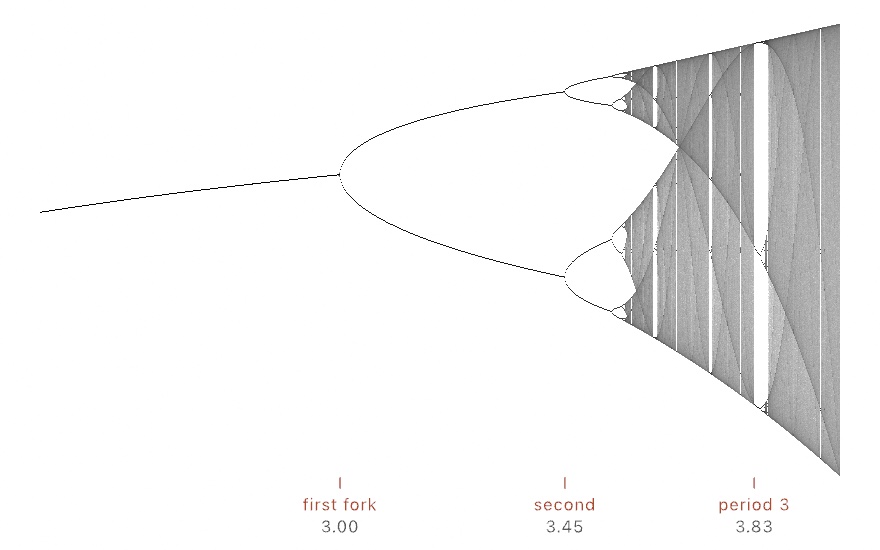
There are two ways to render the same sweep, and both are deterministic:

drawBifurcation(map, over: 3.4...4, in: rect)                 // dots, current fill
let plate = map.bifurcationImage(width: 900, height: 600)     // tonal density image

• drawBifurcation(_:over:in:columns:perColumn:settle:) draws the raw settled values as dots, in the current fill and at the current pointSize, mapped into rect. The default rect is the whole canvas. A translucent fill shades the dense regions darker on its own. The dots export to SVG and PDF as real geometry, so they work on the plotter path. The diagram never changes from frame to frame, so put a heavy one in a retained batch. The data form behind it is bifurcation(over:columns:perColumn:settle:) -> [Vector2], where each point is (r, x).
• bifurcationImage(width:height:over:samplesPerColumn:settle:) bins one long orbit per pixel column, then tones the counts with a single global log factor. Periodic orbits print as crisp dark lines, and chaotic bands print as gray, ink on white. Render it once in setup() and draw it with drawImage.

Both sample the sweep at column centers, never at the range's exact endpoints, because some families are numerically degenerate exactly there. The notes below explain that case. To zoom in, pass a narrower over: range. Try 3.82...3.87, where the period-3 window holds its own complete doubling cascade, which is the whole diagram again in miniature.

The Lyapunov exponent

let l = map.lyapunovExponent(at: 3.9)     // > 0: chaos

The exponent is the average of ln |f′(x)| along the orbit. It is negative where nearby orbits converge, which means a stable cycle. It is positive where they separate exponentially, which is the working definition of chaos. Traced across the sweep window, it dips below zero at every periodic window and touches zero at every fork. For the logistic map it reaches exactly ln 2 at r = 4, and for the tent map it is exactly ln r. The estimate uses the family's analytic derivative when the family has one, and a central difference otherwise. An orbit that visits a point with f′ = 0 is superstable. That visit is floored instead of going to negative infinity, so clamp the trace to your panel when you plot it.

Your own family

You can supply any rule, and the parameter can mean whatever you like:

let ricker = IteratedMap(parameterRange: 1.5...4, valueRange: 0...5, start: 0.5) { x, r in
    x * exp(r * (1 - x))          // the Ricker spawning model
}

Pass derivative: as well if you want exact Lyapunov exponents. Without it, the central difference works well for smooth rules.

Practical notes

• Settle is what makes it a diagram. The sweep discards settle iterations per column, 1000 by default, so only the attractor prints. That is standard practice for these figures. Near a fork the orbit converges very slowly, so a fork can look smeared. When it does, raise settle rather than perColumn.
• Endpoints can be degenerate. The sweep avoids them. At exactly r = 2 a floating-point tent orbit collapses to 0, one doubled bit at a time. At exactly r = 4 the logistic critical orbit dies in two steps. That is why the factories start at 0.3 rather than at the critical point 0.5. Sampling at column centers means a sweep to an endpoint never lands on it.
• The Gauss map's diagram depends on start. Part of its range holds two attractors at once. Sweeping with a different start therefore redraws a stretch of the picture. That is the map behaving correctly, not a bug.
• Costs are small. A full 1080-column image is a few million arithmetic steps, which is milliseconds of setup() work. The one thing to avoid is recomputing a sweep every frame. Keep the Image around, or record the dots into a Batch.

See also Strange attractors for the 2D and 3D members of the family, ChaoticMap and StrangeAttractor. For additive density build-up, see Accumulation. The vector export that the dot form feeds is covered in Export.