Compute & GPU particles

A compute shader is a small program that runs on the GPU over a grid of data. It runs one thread per element, and all the threads run at once. Ollin uses it for the workloads creative coding most wants and the CPU can't reach. It comes in two shapes:

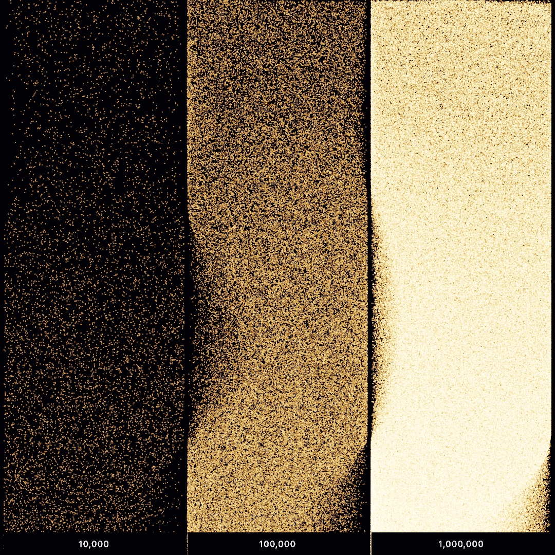
• Buffers hold hundreds of thousands to millions of particles. Each one is updated and drawn on the GPU, so the data never round-trips through the CPU. That is what drives the depth-of-field "sandpainting" look, where faint particles sum as light at counts a draw() loop could never iterate over. The type to start with is Particles.
• Textures hold ping-pong simulations over a 2-D field, such as reaction-diffusion, cellular automata, fluid, and image kernels. Every frame, each cell reads its neighbors and writes the next state on the GPU. The result then draws like any image. The type to start with is Simulation.

In both, you write the per-element update as a short snippet of Metal. Ollin then generates the kernel, owns the double-buffering, and renders the result. One typed core sits under both: ComputeKernel, ComputeBuffer, ComputeTexture, and compute. You can drop down to it for full control.

Compute kernels are written in Metal Shading Language (MSL), a C++-like GPU language. You can write them inline as a Swift string, or keep them in their own .metal file for editor highlighting and checking. Ollin compiles them at runtime, so a kernel you edit hot-reloads with the sketch. The snippets below are MSL, not Swift.

Contents

• Particles - a GPU particle system in a few lines
• The kernel snippet - what's in scope
• The prelude - the shared shader library, spliced into every kernel
• Custom live parameters
• Texture kernels & simulations - Simulation, ComputeTexture
• Kernels in a .metal file
• The typed core - ComputeKernel, ComputeBuffer, compute
• Projecting through the camera - a kernel that sees the sketch's Camera3D
• SpatialHash, the GPU neighbor search
• Notes

Particles

Particles is a GPU particle system. Give it a count and a per-particle update written as a Metal body snippet, then step it and draw it from draw():

import Ollin

@main
final class Flow: Sketch {
    lazy var sand = Particles(count: 1_000_000, step: """
        if (life <= 0.0) {                       // (re)spawn the dead
            position = hash22(float2(float(id), float(u.frameCount))) * u.resolution;
            life = 1.0;
        }
        position += curlNoise(position * 0.002 + u.time * 0.05) * 80.0 * u.dt;
        life -= u.dt;
        color = float4(0.6, 0.8, 1.0, 0.4);
        size = 1.4;
    """)

    override func setup() { toneMap(.aces) }

    override func draw() {
        background(.black)
        blendMode(.add)         // particles sum as light
        stepParticles(sand)   // one GPU simulation step
        drawParticles(sand)     // a million additive discs
    }
}

• stepParticles(_:) records the simulation step, so the kernel runs once over every particle, on the GPU, before the frame is drawn.
• drawParticles(_:) draws the particles as sub-pixel discs. They use the same area-conserving coverage as drawCircle, so a million tiny jittered marks fade by area instead of flickering. The particles composite under the active blendMode, and in draw order with everything else. That means you can draw particles, switch to .normal, and draw a caption over them.

That is the whole loop. For the sandpainting look, pair it with blendMode(.add) and an Accumulator, so the particles sum as light into a running mean that converges. Draw them with the .light style, drawParticles(sand, style: .light), which deposits each particle's light in proportion to its area with no perceptual remap. The default .marks style is ink instead, which is right over a light ground and wrong for a sum of light. Particles at or under one pixel then take a one-texel path, so a million of them cost a million fragments rather than twenty-five million. See Depth of field from light for the deposit rules, and the Examples/Compute/CurlField and Examples/Rendering/DepthOfField examples.

The kernel snippet

In the step: snippet these per-particle fields are locals you read and write:

These names are read-only:

• id is this particle's index (uint).
• u holds the per-frame constants: u.time, u.dt, u.frameCount, u.resolution, u.mouse, u.particleCount.
• custom is a float4 of live parameters you pass to stepParticles.

Particles start zeroed, so life begins at 0, which is why the if (life <= 0.0) spawn pattern above seeds every particle on the first frame.

The prelude

Every kernel gets the shader library spliced in for free. It is the same helper set a fragment Shader gets, so a helper you learn in one works the same way in the other. These are the ones kernels reach for most:

• hash11/hash12/hash13 → float, hash22 → float2, and hash33 → float3 are fast hashes for randomness (hashNM gives N output channels from an M-component seed).
• valueNoise(float2) / valueNoise(float3) → float and fbm(float2) give smooth value noise.
• curlNoise(float2) → float2 is a divergence-free flow field, so particles carried by it swirl without clumping.
• discSample(float2 seed) → float2 is a point in the unit disc, uniform over its area, which is the right scatter for energy-conserving bokeh. ballSample(float3 seed) → float3 is its three-dimensional counterpart, uniform over the unit ball's volume. That is the scatter a lens applies to a sample in camera space.
• ollin_project(camera, world, u.resolution) projects a world point through a Camera3D the sketch packed into the params. See Projecting through the camera.
• srgbToLinear(float3) converts when you need linear color.

The rest of the library is there too (cosine palette, OKLab conversions, the sd* distance-function catalog, the domain operators). See the shader library reference for the full set.

Custom live parameters

You can pass up to four live floats per step, such as a focal distance, a strength, or a mouse-driven parameter. The snippet reads them as custom.x…custom.w:

let focus = mouseIsPressed ? Float(map(mouseX, 0, width, -1, 1)) : 0
stepParticles(sand, custom: SIMD4(focus, 0, 0, 0))

// in the snippet:
float defocus = abs(depth - custom.x);

Texture kernels & simulations

Particles evolves a buffer, and Simulation evolves a 2-D texture instead. The texture is a field where every cell reads its neighbors and writes the next state each frame. That is what drives reaction-diffusion, cellular automata, fluid, and any "ping-pong" sim.

Simulation

Give it a size and a per-cell update written as a Metal body snippet, then step it from draw() and draw its image:

import Ollin

@main
final class RD: Sketch {
    lazy var field = Simulation(width: 512, height: 512, substeps: 12, step: """
        // Gray-Scott reaction-diffusion: chemical A in .r, B in .g.
        float2 lap = -value.xy
            + 0.20 * (tap(-1,0).xy + tap(1,0).xy + tap(0,-1).xy + tap(0,1).xy)
            + 0.05 * (tap(-1,-1).xy + tap(1,-1).xy + tap(-1,1).xy + tap(1,1).xy);
        float a = value.x, b = value.y, reaction = a * b * b;
        float feed = 0.037, kill = 0.06;
        a += 1.0 * lap.x - reaction + feed * (1.0 - a);
        b += 0.5 * lap.y + reaction - (kill + feed) * b;
        result = float4(clamp(a, 0.0, 1.0), clamp(b, 0.0, 1.0), 0.0, 1.0);
    """)

    let seed = ComputeKernel(entry: "seed", """
        kernel void seed(texture2d<float, access::write> dst [[texture(0)]],
                         uint2 gid [[thread_position_in_grid]]) {
            float b = (hash12(float2(gid)) > 0.5 && gid.x > 240 && gid.x < 270) ? 1.0 : 0.0;
            dst.write(float4(1.0, b, 0.0, 1.0), gid);
        }
    """)
    private var seeded = false

    override func draw() {
        if !seeded { compute(seed, writing: field.current); seeded = true }   // initial state
        stepSimulation(field)                                               // one frame of sim
        drawImage(field.image, in: Rectangle(x: 0, y: 0, width: width, height: height))
    }
}

• stepSimulation(_:custom:) records the sim, so substeps kernel iterations run, on the GPU, before the frame is drawn. custom passes up to four live floats, which the snippet reads as custom.x…w.
• field.image wraps the current field as an Image for drawImage. Like any image, it composites in draw order, follows the transform stack, and takes tint. Its texels are treated as linear color, so write sRGB tones through srgbToLinear in the kernel.

In the step: snippet these are in scope:

Fresh fields start zeroed, so seed a sim's initial state on the first frame with a one-shot compute(_:writing: sim.current), as the seeded flag does above. For a full custom kernel signature, use Simulation(width:height:kernel:).

ComputeTexture

A ComputeTexture is the storage behind a sim. It is a persistent 2-D texture that lives on the GPU, and a kernel reads and writes it. Like a ComputeBuffer, it is allocated lazily, so you can construct one with no device, and it starts zeroed. Draw it with its image:

let tex = ComputeTexture(width: 512, height: 512)                 // .rgba16Float by default
let single = ComputeTexture(width: 256, height: 256, format: .r32Float)
// the other formats: .r16Float, .rgba8Unorm, .rgba32Float

You can run a kernel that writes a texture, one thread per texel, with the write texture bound at texture(0). You can also run one that reads one texture and writes another. That is the ping-pong form, where texture(0) is the source and texture(1) is the destination:

// Generate / seed, kernel takes texture2d<…, access::write> [[texture(0)]]:
compute(generator, writing: tex)

// Transform, kernel takes read [[texture(0)]] + write [[texture(1)]]:
compute(blur, reading: src, writing: dst)

The render path may also read the field each frame. In that case, drive a PingPongTexture pair, which is two textures swapped each step. You can also use Simulation, which owns a pair for you.

ComputeTexture.snapshot() reads the float texels back to the CPU for tests and debugging. It works on float formats only.

Kernels in a .metal file

Inline strings are short, but an editor can't highlight or check them. For anything substantial, keep the kernel in its own .metal file, which gets real Metal syntax highlighting and checking. Load it with ComputeKernel(entry:resource:in:):

// Kernels.metal (bundled as a .copy resource on the sketch's target):
//   kernel void blur(texture2d<float, access::read>  src [[texture(0)]],
//                    texture2d<float, access::write> dst [[texture(1)]],
//                    uint2 gid [[thread_position_in_grid]]) { … }

let blur = try ComputeKernel(entry: "blur", resource: "Kernels", in: .module)

The shared types and the shader library are still spliced in. The file references OllinComputeUniforms, hash22, curlNoise, and the rest without writing any #includes. One file can hold any number of kernels, and you load each one by its entry name. They share one compile. Pass in: .module explicitly, because a default would resolve to Ollin's bundle rather than yours. Also list the file as a .copy resource on your target. There is also ComputeKernel(entry:contentsOf:) for an arbitrary file URL. See Examples/Compute/ReactionDiffusion, which keeps its seed and colorize passes in Kernels.metal.

A kernel can write one kind of include. #include "helpers.metal" pulls in another file of your own, resolved against the folder the kernel's source came from. That works exactly as it does for a fragment shader. One helper file can then serve a kernel and a shader, instead of being copied into both.

The typed core

Particles and Simulation are sugar over a public core. Use that core directly for custom particle layouts, custom texture formats, or non-particle compute such as a simulation over your own structs.

ComputeKernel

A ComputeKernel is a Metal kernel function plus its entry name. Write no #includes, because the shared types and the shader library are spliced in for you:

let sim = ComputeKernel(entry: "step", """
    kernel void step(device const MyParticle *inBuf  [[buffer(0)]],
                     device MyParticle       *outBuf [[buffer(1)]],
                     constant OllinComputeUniforms &u [[buffer(10)]],
                     uint i [[thread_position_in_grid]]) {
        if (i >= u.particleCount) { return; }
        MyParticle p = inBuf[i];
        // … your update …
        outBuf[i] = p;
    }
""")

Bind your own buffers at indices 0…9, since compute(_:buffers:) hands a kernel up to ten of them, in order. Index 10 is the standard OllinComputeUniforms, and index 11 is custom, the params. The compiled pipeline is cached by the source's hash, so re-creating the same kernel value each frame costs nothing.

ComputeBuffer

A ComputeBuffer is a persistent, typed GPU buffer. It is the storage a kernel reads and writes each frame. The Metal buffer is allocated lazily, as an Image's texture is, so you can construct a ComputeBuffer anywhere. Fresh buffers start zeroed, so seed one with initial CPU contents through init(_:).

let buffer = ComputeBuffer<MyParticle>(count: 500_000)
let seeded = ComputeBuffer<MyParticle>(initialParticles)   // uploaded once

The render path may read a buffer each frame. For that case, use a PingPong pair, which is two buffers swapped each step. The GPU can then overlap one frame's render with the next step.

compute

Record a dispatch:

// In place, one buffer read and written:
compute(sim, over: buffer)

// Ping-pong, read one and write the other (swap between frames). The two may
// hold different element types: a segment list read, a particle buffer written.
compute(sim, reading: pp.read, writing: pp.write)
pp.swap()

// Up to ten buffers of any element types, bound at indices 0, 1, 2, … in order;
// the thread count defaults to the first buffer's element count.
compute(scatter, buffers: [segments, lookup, particles], count: particles.count, params: params)

// Textures, write one (texture 0), or read one and write another (0 → 1):
compute(generator, writing: tex)
compute(transform, reading: src, writing: dst)

Use the buffers: form for a kernel that reads static geometry uploaded once and writes an OllinParticle buffer the renderer draws. The geometry is a ComputeBuffer of your own struct, and you can bind a table or two beside these buffers. Nothing has to be packed into a struct it isn't. Any ComputeBuffer is a ComputeBindable, whatever its element type.

Draw a ComputeBuffer<OllinParticle> directly with drawParticles(_ buffer:). For a custom struct, draw it with your own geometry, either by reading the buffer in your own shader or by copying the positions out. Draw a ComputeTexture with its image, which is a texture-backed Image.

Projecting through the camera

A kernel can place its particles by projecting world points through the sketch's own Camera3D. A 3D scene sampled on the GPU then lands exactly where drawMesh or project(_:) would put it. cameraParams() packs the active camera's view and projection matrices as the head of a ComputeParams. Those matrices are an OllinCameraMatrices, 128 bytes. Append your own values after the head, and start the kernel's constant struct with the same field:

var params = cameraParams()                                   // the active camera, canvas aspect
params.append(SIMD4<Float>(Float(focalDistance), Float(strength), 0, 0))
compute(scatter, buffers: [segments, particles], params: params)

struct Lens { OllinCameraMatrices camera; float4 lens; };

kernel void scatter(device const Segment *segments [[buffer(0)]],
                    device OllinParticle *out [[buffer(1)]],
                    constant OllinComputeUniforms &u [[buffer(10)]],
                    constant Lens &p [[buffer(11)]],
                    uint id [[thread_position_in_grid]]) {
    float3 world = …;
    float4 screen = ollin_project(p.camera, world, u.resolution);
    if (screen.w <= 0.0) { /* behind the camera */ }
    out[id].position = screen.xy;           // canvas points, top-left origin
    float depth = screen.z;                 // distance along the view axis
}

ollin_project returns the canvas position in xy, the view-space depth in z, and the clip-space w. The depth is positive in front of the camera, and it is the distance a focal plane is measured against. A w of zero or less means the point is behind the camera. You may want to move a point in camera space first, the way a lens pushes a sample sideways and in depth. To do that, take the point through p.camera.view yourself, move it, then finish with ollin_project_eye(p.camera, eye, u.resolution). The matrices are the public Camera3D.viewMatrix and projectionMatrix(aspect:), so ComputeParams.append(camera:aspect:) packs any camera, not only the active one. See Depth of field from light, which builds a lens on this.

SpatialHash, the GPU neighbor search

Every particle-interaction system needs a particle to see the others near it, and the one-thread-per-particle model can't do that on its own. SpatialHash fills that gap. Each frame it sorts the particles into a grid of square cells with a counting sort. The sort counts how many particles land in each cell, then prefix-sums the counts into per-cell start offsets. It then scatters each particle's index into its cell's slot, which leaves buffers a query kernel walks. The cell edge equals the query radius over a toroidal domain, so every neighbor within the radius sits in the queried cell's wrapped 3×3 block.

It drives the built-in artificial-life sims, ParticleLife and PPS, and you can use it directly to write your own. The neighborStep(_:over:reading:writing:) facade builds the hash over your reading particles. It then runs your kernel with the particle buffers and the hash's buffers bound at fixed indices. Your kernel walks the neighbors with the OLLIN_FOR_NEIGHBORS macro, which is spliced into every kernel along with ollin_torus_delta for wrap-correct distances:

let hash = makeSpatialHash(radius: 40, count: 18_000)         // cells over the canvas
let particles = PingPong<OllinParticle>(count: 18_000)     // your own buffers (import COllinShaders)

let step = ComputeKernel(entry: "my_step", """
kernel void my_step(
    device const OllinParticle *inBuf  [[buffer(0)]],
    device OllinParticle       *outBuf [[buffer(1)]],
    device const uint *sortedIdx [[buffer(2)]],
    device const uint *cellStart [[buffer(3)]],
    device const uint *cellCount [[buffer(4)]],
    constant OllinSpatialGrid &grid [[buffer(5)]],
    constant OllinComputeUniforms &u [[buffer(10)]],
    uint id [[thread_position_in_grid]]) {
    if (id >= u.particleCount) { return; }
    OllinParticle p = inBuf[id];
    uint n = 0;
    OLLIN_FOR_NEIGHBORS(p.position, grid, sortedIdx, cellStart, cellCount, j)
        if (j == id) { continue; }
        float2 d = ollin_torus_delta(p.position, inBuf[j].position, grid.worldSize);
        if (length(d) < grid.cellSize) { n++; }
    OLLIN_END_NEIGHBORS
    p.color = float4(float(n) / 12.0, 0.4, 1.0, 1.0);   // color by crowd
    outBuf[id] = p;
}
""")

override func draw() {
    neighborStep(step, over: hash, reading: particles.read, writing: particles.write)
    particles.swap()
    drawParticles(particles.read)
}

A query kernel takes its buffers in a fixed order. reading is at 0, writing at 1, sortedIndices at 2, cellStart at 3, cellCount at 4, and the OllinSpatialGrid at 5, which the hash holds as gridBuffer and whose shape it reports as gridWidth and gridHeight, the cells across and down. Your own buffers follow at 6 and up. ParticleLife binds its interaction matrix at 6. In an export, or while a take plays back, each cell lists its particles in index order. A query that sums over neighbors, a force for example, then adds the same numbers in the same order, and the run repeats. A live frame keeps the order the GPU's threads reached the cell in, which saves a pass. A clock that follows the wall never repeats a run anyway. The neighbor set, and any count of it, is the same either way. See Examples/Compute/NeighborSearch.

Notes

• OllinParticle is the built-in particle struct, with position, velocity, color, size, life, and two scratch floats. drawParticles reads position, color, and size from it. A custom struct that wants the built-in renderer must place those fields at the same offsets. Otherwise it has to render itself.
• Two particle styles. .marks is the default and behaves as ink, with perceptual coverage and an sRGB color. .light behaves as light, with linear area coverage, a linear color, and a one-texel path at or under one pixel. Use .light for anything summed additively into an Accumulator or a noClear canvas. See the light particle style.
• Ping-pong, not in place, for simulation. The kernel may write a buffer or texture that the render path also reads each frame. Drive it as a PingPong or PingPongTexture pair, which Particles and Simulation do for you. In-place compute(_:over:) is for scratch work the render path doesn't also read that frame.
• A ComputeTexture draws as linear color. Its texels feed the render pipeline as linear values, which is the format the renderer composites in. Write display colors in a kernel through srgbToLinear, from the shader library, and keep alpha at 1 for opaque, predictable compositing. Storage is .shared, which is unified memory, with .shaderRead and .shaderWrite usage.
• Determinism. GPU floating-point results are deterministic on a given device, but they can differ across GPUs (reassociation). Compute renders are therefore not pinned to exact reference images.
• Kernels are Metal. They are MSL, compiled at runtime. A syntax error prints to the console and the dispatch is skipped, and the frame still renders. A broken kernel therefore shows as missing particles rather than a crash.

Compute is a core capability, so it ships with import Ollin and needs no satellite.